For each event type, the method with the smallest absolute relative bias among methods that return a point estimate in at least 20 of 200 databases, the usable rate of the package Mack fit, and the best method that also supplies a 95% interval (so its coverage can be read).
Code
elig <- sa |>filter(n_usable >= min_usable, !grepl("_tail$", method), !is.na(rel_bias))pick <- \(d) d |>slice_min(abs(rel_bias), n =1, by = type, with_ties =FALSE)best_any <- elig |>pick()best_int <- elig |>filter(has_interval) |>pick()usable_mack <- sa |>filter(method =="mack") |>select(type, mack_usable = usable_rate)best_any |>select(type, `Best point estimate`= method, `Rel. bias`= rel_bias, `Median signed rel. error`= median_rel_err) |>left_join(best_int |>select(type, `Best with interval`= method, `Bias (interval method)`= rel_bias, Coverage = coverage_usable), by ="type") |>left_join(usable_mack, by ="type") |>mutate(type =factor(type_lab[type], levels = type_lab),across(starts_with("Best"), \(x) method_lab[x])) |>arrange(type) |>rename(Type = type, `Package Mack usable`= mack_usable) |> gt::gt() |> gt::fmt_percent(c(`Rel. bias`, `Median signed rel. error`, `Bias (interval method)`, Coverage, `Package Mack usable`), decimals =0) |> gt::sub_missing(missing_text ="-") |> gt::tab_source_note("Baseline, annual dollar triangles. 'Best' = smallest |relative bias|; this is a descriptive ranking on one simulator, and differences of a few percentage points are within simulation noise. For unauthorized trading the severity tail (shape 0.6) has infinite variance, so a few databases dominate every sum and the median signed error is the steadier statistic.")
Table 1
Type
Best point estimate
Rel. bias
Median signed rel. error
Best with interval
Bias (interval method)
Coverage
Package Mack usable
Trade errors
Mack (package)
1%
3%
Mack (package)
1%
94%
100%
NAV errors
Clark Cape Cod Weibull
0%
0%
Clark Cape Cod Weibull
0%
94%
100%
Unauthorized trading
Frequency x severity
−4%
−29%
Frequency x severity
−4%
63%
0%
Baseline, annual dollar triangles. 'Best' = smallest |relative bias|; this is a descriptive ranking on one simulator, and differences of a few percentage points are within simulation noise. For unauthorized trading the severity tail (shape 0.6) has infinite variance, so a few databases dominate every sum and the median signed error is the steadier statistic.
How to read the table Each row is an event type. The table names the method whose average estimate of the not-yet-found loss came closest to the true amount, and how often the range that method quotes actually contained the truth.
What the table tells you For NAV errors a standard method lands within about 10% of the true missing loss, and for trade errors within about 1%, with its quoted range right roughly nine times in ten. For unauthorized trading, even the best method typically understates the missing loss by 29%, and its quoted range contains the truth only 63% of the time.
Count triangles
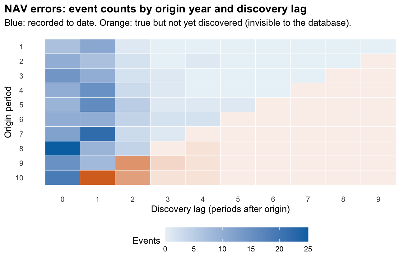
The first question is how many events are still undiscovered. The count triangle has the same shape as the amount triangle but each cell counts events, so it is free of the heavy-tailed severities that make amounts hard.
Code
events <-simulate_database(params, rep =1)sq <-build_square(events, "nav_error", "count", 40, 40, period =4)$squareplot_triangle(sq, "NAV errors: event counts by origin year and discovery lag", "Events")
Figure 1: NAV-error counts, one simulated database, annual granularity.
How to read the plot This is the same triangle as on the Overview page, but each box counts events instead of dollars. Each row is a year in which events happened, each column is how many years later they were found, and the fainter orange boxes are events not yet found.
What the plot tells you The pattern is the same as for dollars: recent years show few recorded events only because many have not been found yet, so a raw count of recent events understates what has really happened.
The target is the number of events inside the development window that are not yet discovered. Methods that need a tail beyond the window are not applied to counts.
Code
score_gt(s, "count")
Table 2
Method
Usable (of 200)
Failed
Suspect
Rel. bias
Median signed rel. error
Coverage (usable fits)
Coverage (all fits)
Recent-origin bias
Trade errors
Chain-ladder (vol-weighted)
200
0
0
1%
2%
-
-
1%
Mack (package)
200
0
0
1%
2%
92%
92%
1%
Bootstrap
200
0
0
1%
3%
86%
86%
1%
Clark LDF loglogistic
0
0
200
-
-
-
-
-
Clark LDF Weibull
200
0
0
102%
21%
54%
54%
14%
NAV errors
Chain-ladder (vol-weighted)
200
0
0
4%
2%
-
-
5%
Mack (package)
200
0
0
4%
2%
96%
96%
5%
Bootstrap
200
0
0
6%
5%
96%
96%
7%
Clark LDF loglogistic
189
0
11
13%
14%
91%
86%
9%
Clark LDF Weibull
200
0
0
1%
0%
97%
97%
3%
Unauthorized trading
Chain-ladder (vol-weighted)
200
0
0
19%
−36%
-
-
19%
Mack (package)
0
200
0
-
-
-
-
-
Bootstrap
0
0
200
-
-
-
-
-
Clark LDF loglogistic
0
200
0
-
-
-
-
-
Clark LDF Weibull
0
200
0
-
-
-
-
-
Relative bias = sum(estimate - truth) / sum(truth) over usable fits. Coverage (usable fits) = share of usable fits whose 95% interval contains the truth; Coverage (all fits) counts failed, suspect and interval-free fits as misses. Recent-origin bias = relative bias restricted to the most recent origin period (latest 4 quarters). Failed or suspect fits are excluded from bias. A dash means fewer than 20 usable fits (not interpretable) or no interval.
How to read the table Each block is an event type and each row a method for estimating how many events are still undiscovered. “Rel. bias” is the average over- or under-estimate (positive means too high), and “Coverage” is how often the method’s 95% range contained the true count.
What the table tells you Counting missing events is the easy part where events are plentiful: standard methods are within about 1% for trade errors and 4% for NAV errors. For unauthorized trading, which averages about one event a year, the standard method fails in all 200 databases because there is too little data.
Code
plot_errors(res$reps, "count")
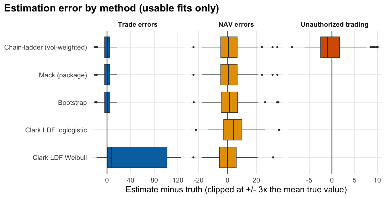
Figure 2
How to read the plot Each box shows how far the estimated number of missing events was from the truth across the 200 simulated databases; the vertical line at zero is a perfect estimate, and a narrower box means a more dependable method.
What the plot tells you For trade and NAV errors the boxes sit tightly around zero, so standard methods count missing events reliably. For unauthorized trading only the simplest method produces a count at all, and it is typically 36% too low, so the loss history alone cannot be trusted for that event type.
Code
sc <- s |>filter(kind =="count", scenario =="baseline", granularity =="annual")get <- \(t, m, col) sc[[col]][sc$type == t & sc$method == m]
Trade errors (many events, fast discovery): Mack and Bootstrap are close to unbiased (relative bias 1% and 1%).
NAV errors: Mack relative bias 4%, interval coverage 96%.
Unauthorized trading (about one event a year): Mack is usable in 0 of 200 databases. With so few events, a count triangle has too little data for development factors; the chain-ladder point estimate is available but has no interval.
Quarterly triangles (40 x 40) are far sparser; see Method validation for the usable-fit rates.
Dollar-loss triangles
Dollar-loss triangles are what a risk committee cares about, but they are the hard case: a single large event dominates a cell, and late-discovered events are larger.
Routes to the missing amount
Direct development methods on the dollar triangle: plain chain-ladder, Mack (the package implementation, and a version that sets development factors of empty columns to 1 so it runs on sparse triangles), Mack using only the latest three calendar diagonals, bootstrap chain-ladder, and Clark growth curves.
Bornhuetter-Ferguson (BF) and Benktander. An a-priori expected loss (loss per unit exposure, estimated from the five oldest origin years, times exposure) is weighted by the share still unreported. The share comes either from the triangle’s own chain-ladder pattern, or from an external benchmark pattern. The benchmark here is the generator’s own lag distribution, so it shows what an accurate external pattern buys and is optimistic. BF and Benktander give point estimates only.
Frequency x severity: project the number of undiscovered events from the count triangle, then price each projected event by resampling observed severities at a similar lag. This keeps the stable count signal separate from the noisy severities. It ignores parameter uncertainty, so we expect its intervals to be too narrow. A variant pools all observed severities and re-applies an estimated linear lag uplift.
The target is the undiscovered loss inside the 10-year window. The one tail-extrapolating method (Clark with a tail) is scored against the total including loss beyond the window.
Code
score_gt(s, "amount")
Table 3
Method
Usable (of 200)
Failed
Suspect
Rel. bias
Median signed rel. error
Coverage (usable fits)
Coverage (all fits)
Recent-origin bias
Trade errors
Chain-ladder (vol-weighted)
200
0
0
1%
3%
-
-
2%
Mack (package)
200
0
0
1%
3%
94%
94%
2%
Mack (empty columns = 1)
200
0
0
1%
3%
94%
94%
2%
Mack (latest 3 diagonals)
200
0
0
4%
7%
88%
88%
4%
Bornhuetter-Ferguson
200
0
0
2%
3%
-
-
3%
Benktander
200
0
0
2%
3%
-
-
2%
BF (benchmark pattern)
200
0
0
2%
6%
-
-
2%
Benktander (benchmark pattern)
200
0
0
2%
5%
-
-
2%
Bootstrap
200
0
0
2%
4%
86%
86%
2%
Clark LDF loglogistic
0
0
200
-
-
-
-
-
Clark LDF Weibull
200
0
0
94%
41%
54%
54%
14%
Clark LDF loglogistic + tail
0
0
200
-
-
-
-
-
Clark Cape Cod Weibull
200
0
0
254%
257%
0%
0%
35%
Frequency x severity
200
0
0
−2%
−1%
92%
92%
−1%
Frequency x severity (pooled, uplift)
200
0
0
6%
8%
94%
94%
7%
NAV errors
Chain-ladder (vol-weighted)
200
0
0
10%
−3%
-
-
7%
Mack (package)
200
0
0
10%
−3%
92%
92%
7%
Mack (empty columns = 1)
200
0
0
10%
−3%
92%
92%
7%
Mack (latest 3 diagonals)
200
0
0
12%
2%
86%
86%
11%
Bornhuetter-Ferguson
200
0
0
7%
2%
-
-
4%
Benktander
200
0
0
7%
−2%
-
-
4%
BF (benchmark pattern)
200
0
0
3%
4%
-
-
4%
Benktander (benchmark pattern)
200
0
0
1%
3%
-
-
3%
Bootstrap
200
0
0
14%
2%
90%
90%
10%
Clark LDF loglogistic
197
0
3
14%
11%
89%
88%
10%
Clark LDF Weibull
200
0
0
2%
−5%
90%
90%
4%
Clark LDF loglogistic + tail
197
0
3
124%
30%
89%
88%
31%
Clark Cape Cod Weibull
200
0
0
0%
0%
94%
94%
3%
Frequency x severity
200
0
0
−7%
−6%
90%
90%
−1%
Frequency x severity (pooled, uplift)
200
0
0
22%
8%
88%
88%
20%
Unauthorized trading
Chain-ladder (vol-weighted)
200
0
0
866%
−42%
-
-
2,641%
Mack (package)
0
200
0
-
-
-
-
-
Mack (empty columns = 1)
200
0
0
866%
−42%
43%
40%
2,641%
Mack (latest 3 diagonals)
200
0
0
290%
−54%
37%
29%
421%
Bornhuetter-Ferguson
200
0
0
70%
−15%
-
-
70%
Benktander
200
0
0
73%
−2%
-
-
66%
BF (benchmark pattern)
200
0
0
50%
14%
-
-
80%
Benktander (benchmark pattern)
200
0
0
27%
28%
-
-
68%
Bootstrap
0
0
200
-
-
-
-
-
Clark LDF loglogistic
0
200
0
-
-
-
-
-
Clark LDF Weibull
0
200
0
-
-
-
-
-
Clark LDF loglogistic + tail
0
200
0
-
-
-
-
-
Clark Cape Cod Weibull
0
200
0
-
-
-
-
-
Frequency x severity
200
0
0
−4%
−29%
63%
63%
26%
Frequency x severity (pooled, uplift)
200
0
0
24%
−17%
67%
67%
43%
Relative bias = sum(estimate - truth) / sum(truth) over usable fits. Coverage (usable fits) = share of usable fits whose 95% interval contains the truth; Coverage (all fits) counts failed, suspect and interval-free fits as misses. Recent-origin bias = relative bias restricted to the most recent origin period (latest 4 quarters). Failed or suspect fits are excluded from bias. A dash means fewer than 20 usable fits (not interpretable) or no interval.
How to read the table This is the same layout as the count table, but for dollars of undiscovered loss. A dash means a method worked in fewer than 20 of the 200 databases, or does not quote a range, so its bias or coverage is not reported.
What the table tells you For trade and NAV errors most standard methods are within about 15% of the truth, though the growth-curve methods (Clark) can be far off. For unauthorized trading the package version of Mack produces no answer in any database, and the version forced to run overstates the average by 866% while its range holds the truth only 43% of the time.
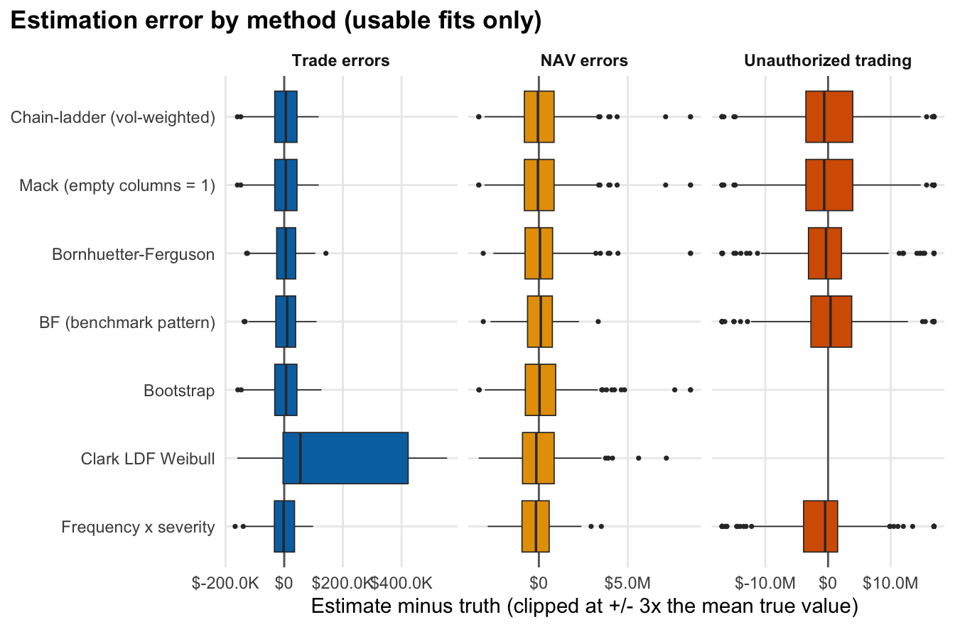
How to read the plot Each box shows how far the estimated dollar loss was from the truth across the 200 simulated databases, for each method and event type. The vertical line at zero is a perfect estimate, boxes to the right overstate the loss, and wider boxes mean less dependable estimates.
What the plot tells you Where events are frequent the boxes are narrow and centred near zero, so the loss estimate is dependable. For unauthorized trading they are wide and lopsided: a method can be badly wrong in one database and right in the next, so a single estimate should be read as a rough range, not a point.
Trade and NAV errors: Mack, bootstrap, Bornhuetter-Ferguson and frequency x severity are all usable and within about 15% of the truth in aggregate. Relative biases for NAV errors are Mack 10%, bootstrap 14%, BF with its own pattern 7% and frequency x severity -7%.
Package Mack versus Mack with empty-column handling. The package fails in 200 of 200 unauthorized-trading databases (non-finite development factors from empty columns). Setting those factors to 1 makes it run in 200 of them, and identical to the package where the package runs (trade and NAV errors). So the failure is an implementation limit. But the result when it runs is poor: relative bias 866%, median signed error -42% and interval coverage 43%. A single large loss in the latest diagonal is multiplied by large factors, so the mean is far too high while the typical database is underestimated.
Bornhuetter-Ferguson on unauthorized trading does not remove the problem. With its own pattern the relative bias is 70% (median -15%); with the benchmark pattern 50% (median 14%). The a-priori loss per unit exposure is itself estimated from heavy-tailed history, so one large old loss inflates every origin year. BF has no interval here.
Frequency x severity has relative bias -4% on unauthorized trading and the best coverage among methods with intervals, but only 63%. At long lags few observed events exist: 62% of projected unauthorized-trading events are priced from the all-event pool because no events are nearby in lag (median fewest donors for any lag with projected events: 2). The uplift-pooling variant has relative bias 24% and coverage 67%, so pooling does not by itself fix the under-coverage.
Recent-origin bias (relative bias for the latest origin year only) is much larger than overall bias for unauthorized trading with frequency x severity (26% against -4% overall): the most recent origin year has the largest undiscovered share, so errors concentrate there, and it is exactly the year a decision-maker cares about.
Beyond the window: about 40% of the true undiscovered unauthorized-trading loss is discovered more than 40 quarters after origin, although only 2.7% of unauthorized-trading events are (late events are scaled up by the severity-growth term). No in-window method can see it; it needs an explicit tail assumption.
Method settings
Bootstrap:BootChainLadder with R = 1000 resamples and process.distr = "gamma". Re-running trade and NAV errors with "od.pois" on the first 100 databases gives practically the same bias and coverage, so this choice is not what drives the under-coverage.
How to read the table The table compares two technical settings of the same bootstrap method on trade and NAV errors, showing average bias and how often its range contained the truth.
What the table tells you The choice of setting makes no practical difference, so the bootstrap’s ranges being somewhat too narrow is not an artifact of how it was configured.
Clark curves: ages are period ends (1 to 10 years), the package default for the average date of loss (half an origin period), maxage is the window length, and Cape Cod exposure is the exposure path scaled so that expected loss ratios start near 1. These conventions are the package’s own; they are not the cause of the poor trade-error results. The cause is the shape of the data. About 100% of trade-error loglogistic fits end on the optimiser bound: the package restricts the loglogistic scale (the age by which half the loss is reported) to be at least half a year here, but most trade-error loss is already reported in the first period. The Weibull Cape Cod fit converges to a degenerate curve (median shape 0.09, scale 3.8 years) in 100% of trade-error databases, which implies a long thin tail that the oldest origin years do not show. That is a fit to the wrong shape, not exposure scaling, and the resulting 254% bias stands.
Method validation
Because the data are synthetic, every method can be scored against the true undiscovered amount. We generate 200 independent databases per scenario, fit each method to each, and record bias, error and interval coverage. A fit is usable only if the method ran and passed sanity checks. Fits that error out (failed) or return an implausible result (suspect, for example a bootstrap IBNR of zero, a bootstrap mean below 10% of the deterministic chain-ladder, or a growth-curve parameter on its optimiser bound) are excluded from bias figures. Two coverage columns are shown: coverage among usable fits, and coverage over all fits where failed, suspect and interval-free fits count as misses. Rows with fewer than 20 usable fits are shown as a dash.
These are tests of how methods behave under this simulator, not proof of how they behave on any real firm’s data.
Scorecard: dollar losses (baseline, annual triangles)
Code
plot_scorecard(s, "amount")
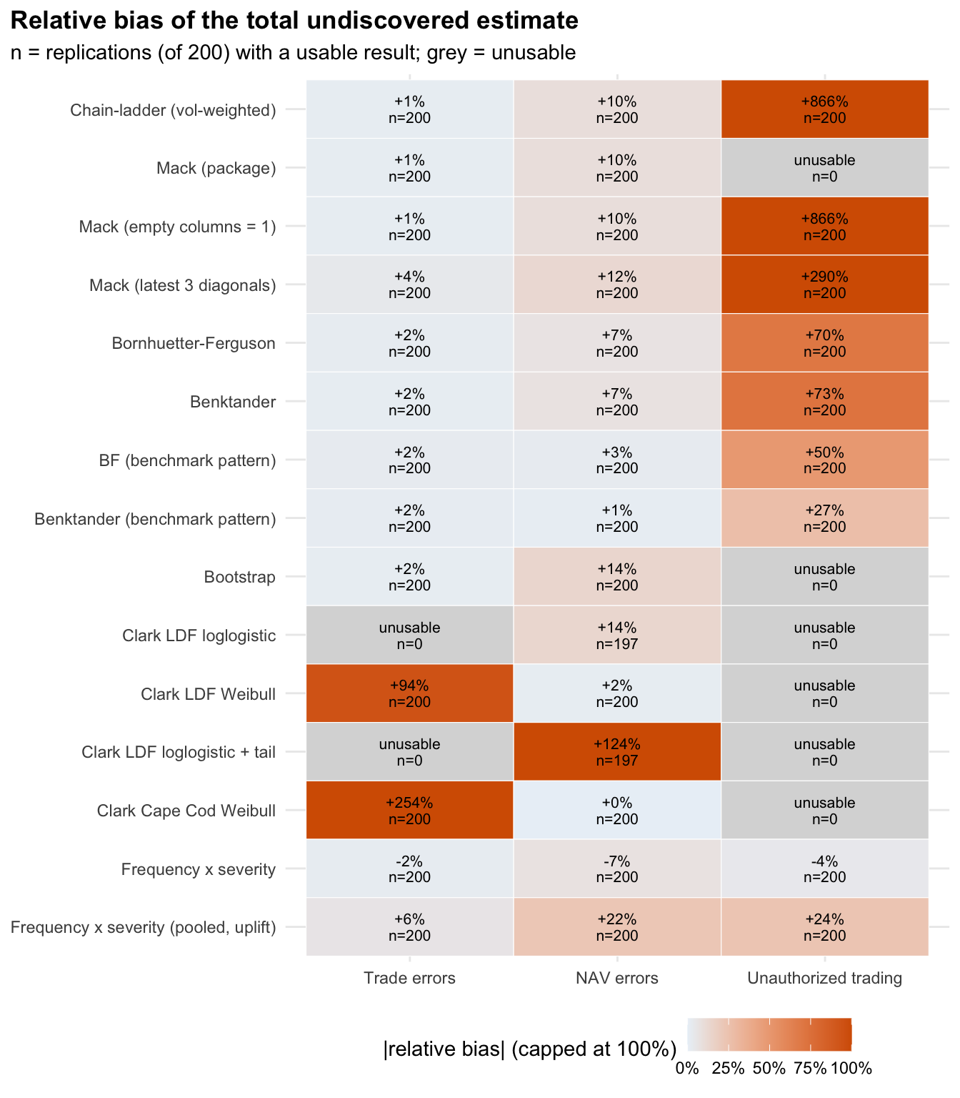
Figure 4
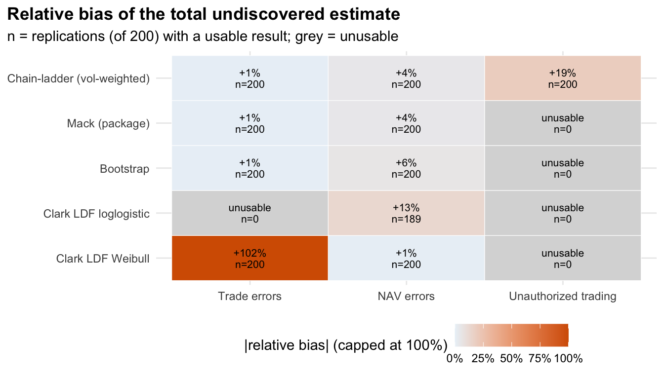
How to read it Each tile is one method for one event type. The number is the average over- or under-estimate, “n” is how many of the 200 databases the method produced a usable answer for, darker orange means further from the truth, and grey means the method could not be used.
What it tells you No method is dependable for all three event types. The unauthorized-trading column is mostly grey or dark orange, so choosing the right method for each event type matters more than choosing one method for the firm.
Scorecard: event counts
Code
plot_scorecard(s, "count")
Figure 5
How to read the plot This is the same scorecard as above, but for counts of missing events instead of dollars.
What the plot tells you Counts are estimated reliably for trade and NAV errors, but for unauthorized trading only the simplest method produces a count at all, which confirms that the difficulty with that event type is how rare it is.
Interval coverage
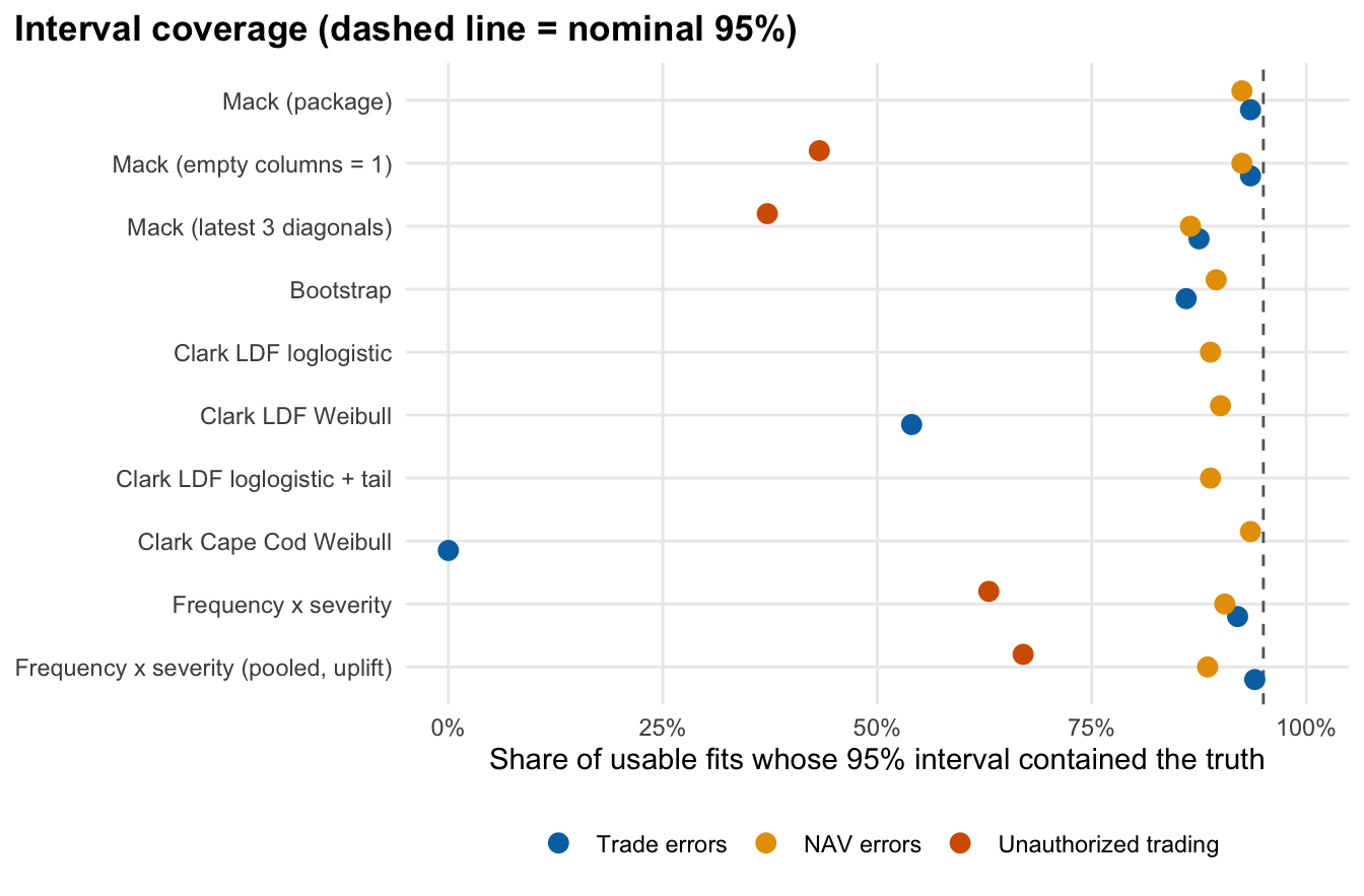
A well-calibrated 95% interval should contain the truth about 95% of the time. Methods whose intervals are narrower than the true uncertainty fall left of the dashed line. BF and Benktander give no interval and are not shown.
Code
plot_coverage(s, "amount")
Figure 6
How to read the plot Each dot shows how often a method’s quoted 95% range actually contained the true loss. The dashed line at 95% is where an honest range should sit, and dots to the left mean the range is too narrow.
What the plot tells you Every dot sits at or left of the dashed line, and many are well to the left, so the ranges these methods quote are optimistic and should be widened before being used for a decision. For unauthorized trading the best available method covers the truth only 63% of the time.
Annual vs. quarterly triangles
Finer triangles contain more empty cells. The share of fits that were usable:
How to read the table The table shows the share of databases in which each method produced a usable answer, using yearly data (a 10 x 10 table) and quarterly data (a 40 x 40 table).
What the table tells you Finer data is not better for the standard methods: for NAV errors the standard package methods work on yearly data but fail completely on quarterly data, because many cells are empty. Use yearly data unless the loss history is very large.
Why fits fail
Code
res$reps |>filter(scenario =="baseline", kind =="amount", granularity =="annual", status %in%c("failed", "suspect")) |>mutate(reason =case_when(grepl("NA/NaN/Inf", message) ~"Package error: non-finite development factor (empty column)",grepl("optimiser bound", message) ~"Growth-curve parameter at optimiser bound",grepl("bootstrap mean IBNR", message) ~"Bootstrap returned ~0 where chain-ladder does not",grepl("zero", message) ~"Bootstrap mean IBNR is zero",grepl("error in evaluating", message) ~"Package error inside growth-curve fit",TRUE~substr(message, 1, 60) )) |>count(Type =factor(type_lab[type], levels = type_lab), Method = method_lab[method], Status = status, Reason = reason, name ="Fits") |>arrange(Type, desc(Fits)) |> gt::gt(groupname_col ="Type") |> gt::tab_source_note("Baseline, annual, dollar triangles; 200 databases per event type, so counts within a type are out of 200 per method.")
Table 6
Method
Status
Reason
Fits
Trade errors
Clark LDF loglogistic
suspect
Growth-curve parameter at optimiser bound
200
Clark LDF loglogistic + tail
suspect
Growth-curve parameter at optimiser bound
200
NAV errors
Clark LDF loglogistic
suspect
Growth-curve parameter at optimiser bound
3
Clark LDF loglogistic + tail
suspect
Growth-curve parameter at optimiser bound
3
Unauthorized trading
Bootstrap
suspect
Bootstrap returned ~0 where chain-ladder does not
200
Clark Cape Cod Weibull
failed
Package error inside growth-curve fit
200
Clark LDF Weibull
failed
Package error inside growth-curve fit
200
Clark LDF loglogistic
failed
Package error inside growth-curve fit
200
Clark LDF loglogistic + tail
failed
Package error inside growth-curve fit
200
Mack (package)
failed
Package error: non-finite development factor (empty column)
200
Baseline, annual, dollar triangles; 200 databases per event type, so counts within a type are out of 200 per method.
How to read the table Each row counts how often a method failed or was flagged as unreliable, and the reason, for the baseline case.
What the table tells you Failures are systematic, not random: they come from empty development columns in sparse data and from fitted curves that hit the limits of what the software allows. That is a warning that the data are too thin for the method, not a sign of a one-off error.
Reading the results
No method is reliable for every event type. The ranking changes with how many events there are and how heavy their tails are.
The standard development methods (Mack, bootstrap) are trustworthy where events are plentiful (trade errors) and acceptable where they are moderately frequent (NAV errors). Their intervals are somewhat too narrow even there.
For rare, heavy-tailed events (unauthorized trading), the package Mack cannot run, and once it is made to run it is badly biased with poor coverage. Bornhuetter-Ferguson with an external pattern and frequency x severity are the most defensible point estimates here, but all methods are unstable and none has well-calibrated intervals.
Stress tests
Chain-ladder methods assume that the pattern of past development carries forward. Five scenarios break that assumption, or the data-generating assumptions, in different ways. All use annual triangles and the same 200 seeds as the baseline (the scenario index is part of the seed, so each scenario has its own databases).
Scenario
Why it is hard
Heavy-tail shock
Two very large unauthorized-trading losses are injected; one is discovered, one is not yet (table below)
Control improvement
Detection gets faster partway through, so history over-predicts future development
Exposure growth
Rising volume distorts comparisons across origin periods
Overdispersion
Negative-binomial counts (same mean as baseline, larger variance)
Reporting threshold $10k
Losses below $10,000 are never recorded, as in many real loss databases
Heavy-tail shock: what is injected
Code
n_o <- params$horizon$n_origininj <-load_params()$scenarios$heavy_tail_shock$injected_eventstibble(`Event`=seq_along(inj),`Origin quarter`=map_dbl(inj, "origin"),`Lag (quarters)`=map_dbl(inj, "lag"),`Discovery quarter`=`Origin quarter`+`Lag (quarters)`,Severity =map_dbl(inj, "severity")) |>mutate(`Discovered by quarter 40?`=if_else(`Discovery quarter`<= n_o, "Yes (in the realised history)", "No (undiscovered at evaluation)")) |> gt::gt() |> gt::fmt_currency(Severity, decimals =0, suffixing =TRUE)
Table 7
Event
Origin quarter
Lag (quarters)
Discovery quarter
Severity
Discovered by quarter 40?
1
12
15
27
$60M
Yes (in the realised history)
2
20
22
42
$40M
No (undiscovered at evaluation)
How to read the table The table lists the two very large unauthorized-trading losses added to the stress scenario: when each happened, how long until discovery, and whether it was found by the end of the history.
What the table tells you One loss was found inside the history and one was not: the second is discovered after the evaluation date, so it is part of the true undiscovered loss that no method could have seen in the data.
The undiscovered truth in this scenario is therefore mainly the second injected loss: it is not in the realised history, so a method cannot see it in the severity pool.
Control improvement: what the shift does
Code
shift <-load_params()$scenarios$control_improvement$control_shiftcq <- shift$calendar_quarterpairs <-map(1:40, \(r) { before <-simulate_database(apply_scenario(load_params(), "baseline"), rep = r) |>filter(type =="trade_error")set.seed(r)list(before = before, after =apply_control_shift(before, shift))})both <- \(f) c(Baseline =mean(map_dbl(pairs, \(p) f(p$before, p$before))), `After shift`=mean(map_dbl(pairs, \(p) f(p$before, p$after))))# f(before, after) is evaluated on `after` and may use `before` to select the same eventsrows <-list("Mean lag, all events (quarters)"=both(\(b, e) mean(e$lag)),"Mean lag, events originating after the shift (quarters)"=both(\(b, e) mean(e$lag[b$origin > cq])),"Mean time remaining after the shift quarter, events pending at that quarter (quarters)"=both(\(b, e) mean((e$origin + e$lag - cq)[b$origin <= cq & b$origin + b$lag > cq])),"Share of events undiscovered at quarter 40"=both(\(b, e) mean(e$origin + e$lag > n_o)))tibble(Measure =names(rows), Baseline =map_dbl(rows, "Baseline"), `After shift`=map_dbl(rows, "After shift")) |>mutate(Change =`After shift`/ Baseline -1) |> gt::gt() |> gt::fmt_number(c(Baseline, `After shift`), decimals =3) |> gt::fmt_percent(Change, decimals =0) |> gt::tab_source_note("Trade errors, first 40 baseline databases, with the shift applied to the same events (paired). Time remaining is measured from the later of the shift quarter and the event's origin, and rounded stochastically.")
Table 8
Measure
Baseline
After shift
Change
Mean lag, all events (quarters)
0.477
0.358
−25%
Mean lag, events originating after the shift (quarters)
0.483
0.242
−50%
Mean time remaining after the shift quarter, events pending at that quarter (quarters)
2.045
1.024
−50%
Share of events undiscovered at quarter 40
0.014
0.007
−49%
Trade errors, first 40 baseline databases, with the shift applied to the same events (paired). Time remaining is measured from the later of the shift quarter and the event's origin, and rounded stochastically.
How to read the table The table compares the same trade errors before and after the control improvement, showing how long they take to be found.
What the table tells you The improvement does what it is meant to: events originating after it are found in about half the time, and the share of events still undiscovered at the end of the history falls by about half. This is the real change that the estimation methods are then asked to detect.
Mean estimate vs. mean truth
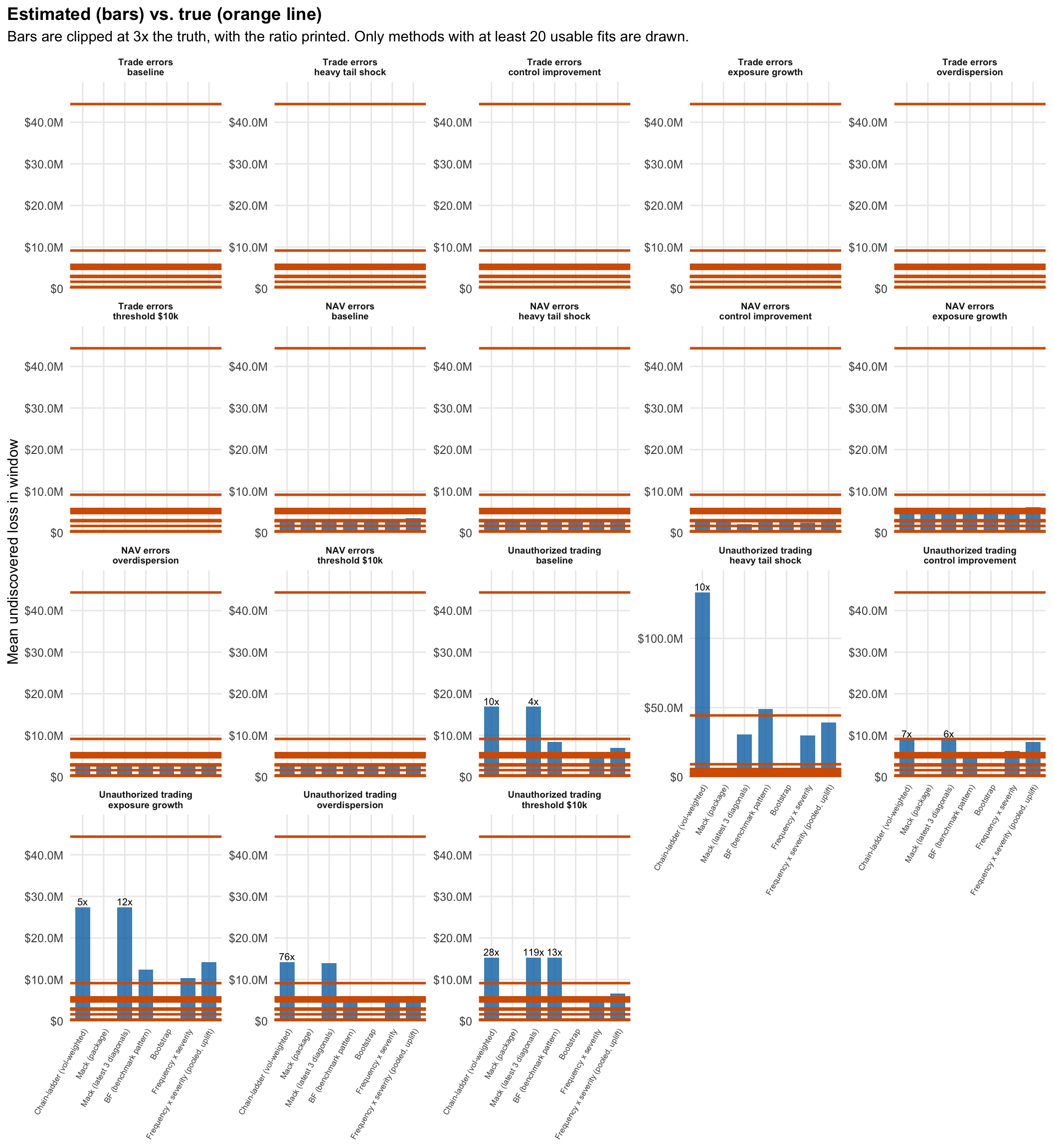
Relative errors explode when the true value is near zero, so this page shows absolute dollars: the mean undiscovered loss in the window, true and estimated, for the methods that run. Methods with fewer than 20 usable fits are omitted. “Mack, latest 3 diagonals” restricts development factors to the three most recent calendar diagonals, a standard remedy when development changes over calendar time; the “benchmark pattern” BF uses an externally supplied development pattern from the baseline generator, so it does not adapt to a changed pattern either.
Code
d <-stress_means(res$reps) |>filter(n >= min_usable)truth <- d |>distinct(scenario, type, Truth)d_plot <- d |>mutate(shown =pmin(Estimate, 3* Truth), label =if_else(Estimate >3* Truth, sprintf("%.0fx", Estimate / Truth), NA_character_),panel =paste0(type, "\n", str_replace_all(as.character(scenario), c("reporting_threshold_10k"="threshold $10k", "_"=" "))),panel =factor(panel, levels =unique(panel[order(type, scenario)])))ggplot(d_plot, aes(method, shown)) +geom_col(fill ="#0072B2", alpha =0.8, width =0.7) +geom_text(aes(label = label), vjust =-0.3, size =2.6, na.rm =TRUE) +geom_hline(data = truth, aes(yintercept = Truth), colour ="#D55E00", linewidth =0.9) +facet_wrap(vars(panel), scales ="free_y", ncol =5) +scale_y_continuous(labels = fmt_usd, expand =expansion(mult =c(0, 0.12))) +scale_x_discrete(guide =guide_axis(angle =60)) +labs(x =NULL, y ="Mean undiscovered loss in window",title ="Estimated (bars) vs. true (orange line)",subtitle ="Bars are clipped at 3x the truth, with the ratio printed. Only methods with at least 20 usable fits are drawn.") +theme_op() +theme(axis.text.x =element_text(size =6), strip.text =element_text(size =7))
Figure 7
How to read the plot Each panel is one event type under one scenario. Blue bars are each method’s average estimate of the undiscovered loss, the orange line is the true amount, and bars are cut off at three times the truth with the ratio printed.
What the plot tells you When nothing changes, bars sit on the orange line. After a control improvement the standard methods overstate trade errors by 62% because they assume the old, slower detection still applies, while using only the latest three diagonals of data brings the estimate close to the truth.
How to read the table The table lists the same stress results in dollars: the true undiscovered loss, each method’s average estimate, and the error (estimate minus truth).
What the table tells you The errors are small for trade and NAV errors in most scenarios and large for unauthorized trading, where the standard chain-ladder method can overstate the loss many times over. This is why a firm should not rely on one method for rare, large events.
Can a calendar-diagonal test see the change?
A simple diagnostic: the standardised age-to-age residuals on the latest two calendar diagonals, summed as a z-score. A strongly negative value means recent development is below what earlier years predicted. The table shows how often the test (z below -1.645) fires in each scenario.
How to read the table The table shows how often a simple alarm, which compares the latest two years of development with earlier years, signals that detection has changed.
What the table tells you The alarm rarely fires when nothing has changed, but it also catches the real control improvement in only 32% of trade-error databases and 12% of NAV-error databases. A firm should not wait for a statistical alarm before checking whether an improved control has changed its loss pattern.
Control improvement. After detection speeds up, the true undiscovered trade-error amount falls from $185.0K to $94.5K, about half. Methods trained on the earlier, slower history keep projecting the old development: Mack’s mean estimate is $153.4K, 62% too high. A firm that has just improved its controls will over-reserve if it applies old development factors. Restricting the factors to the latest three diagonals removes most of the error here ($96.2K against the truth) and reduces it for NAV errors ($2.1M against $1.6M), at the price of noisier factors in the other scenarios (4% bias and 88% coverage for trade errors in the baseline, against 1% and 94%). It does not help unauthorized trading. The calendar-diagonal test is weak on 10 x 10 annual triangles: it flags the change in 32% of trade-error databases and 12% of NAV-error databases, against about 0% false alarms in the baseline. A change that the test cannot see on annual data can still be large enough to matter.
Heavy-tail shock. For unauthorized trading, frequency x severity has relative bias -33% and interval coverage 94%. BF with a benchmark pattern is close in aggregate (11%), and plain chain-ladder is wildly high because the injected losses are multiplied by large development factors. One injected loss is discovered inside the realised history and one is not (table above), so part of the truth is information the severity pool never contained.
Exposure growth. Moderate growth changes little for the event types where the methods already work.
Overdispersion. Interval coverage falls for the methods that have intervals: Mack covers 90% of trade-error databases and bootstrap 78%, against 94% and 86% in the baseline. Clustered or overdispersed counts make the stated 95% intervals less trustworthy.
Reporting threshold. A $10k threshold removes most trade errors from the database (the true undiscovered trade-error amount falls from $185.0K to $80.0K) while NAV errors and unauthorized trading are barely affected; for trade and NAV errors the standard methods still work on what remains (unauthorized-trading means are dominated by a few databases and vary a lot between scenarios).