All data are simulated. No internal or client loss data are used, and every parameter is an assumption chosen for plausibility, stored in params.yaml. The point is to have a known ground truth against which estimation methods can be scored, not to describe a real firm.
Generator design
For each event type and origin quarter:
Count ~ Poisson(\(\lambda \times \text{exposure}\)), where exposure grows 1.0% per quarter. Counts are independent across quarters and event types, with no overdispersion or clustering (see Limitations).
Discovery lag (quarters): a mixture of a fast component (geometric) and a slow component (discretised lognormal).
Severity: lognormal body spliced to a generalised Pareto tail, then scaled by \((1 + e \times \text{lag})\), so events found later are larger. The uplift is linear in the lag (not compounding). It is a crude stand-in for an unauthorized position that keeps growing while hidden; \(e\) is the only mechanism by which a loss can change while undiscovered, so every dollar figure for controls on the Control Value page scales with it.
The loss is recorded in full at the discovery date.
The generator keeps the full square, so the true undiscovered loss is always known.
Parameters
Code
tibble(`Event type`= type_lab[types],`Events / qtr`=map_dbl(params$event_types, "lambda"),`Fast-lag weight`=map_dbl(params$event_types, \(x) x$lag$w_fast),`Slow-lag median (qtrs)`=map_dbl(params$event_types, \(x) exp(x$lag$slow_meanlog)),`Median lag (qtrs)`= lag_stats$median[match(type_lab[types], lag_stats$type)],`90th-pct lag (qtrs)`= lag_stats$p90[match(type_lab[types], lag_stats$type)],`Median severity`=map_dbl(params$event_types, \(x) exp(x$severity$meanlog)),`Tail prob.`=map_dbl(params$event_types, \(x) x$severity$p_tail),`Severity uplift per lag qtr (linear, e)`=map_dbl(params$event_types, \(x) x$severity$lag_elasticity)) |> gt::gt() |> gt::fmt_currency(`Median severity`, decimals =0) |> gt::fmt_number(c(`Events / qtr`, `Slow-lag median (qtrs)`), decimals =1) |> gt::fmt_number(c(`Fast-lag weight`, `Tail prob.`, `Severity uplift per lag qtr (linear, e)`), decimals =2) |> gt::tab_source_note("All values are judgement-based assumptions (status: assumption in params.yaml), with no calibration to public loss data. Total expected loss is checked against a 10-15 bps of AUM target in the sanity check below; plausible ranges are given beside each value in params.yaml.")
Table 1
Event type
Events / qtr
Fast-lag weight
Slow-lag median (qtrs)
Median lag (qtrs)
90th-pct lag (qtrs)
Median severity
Tail prob.
Severity uplift per lag qtr (linear, e)
Trade errors
60.0
0.85
1.6
0
1
$2,441
0.03
0.02
NAV errors
6.0
0.50
4.5
2
9
$29,733
0.05
0.05
Unauthorized trading
0.3
0.10
7.4
6
22
$242,802
0.08
0.08
All values are judgement-based assumptions (status: assumption in params.yaml), with no calibration to public loss data. Total expected loss is checked against a 10-15 bps of AUM target in the sanity check below; plausible ranges are given beside each value in params.yaml.
How to read the table Each row is an event type. The columns show how often events occur, how many quarters they typically take to be found (median and 90th percentile), how large they are, and how much their size grows for each quarter they stay hidden.
What the table tells you The three event types are very different risks. Trade errors are frequent (about 60 a quarter) and small, and are found at once, while unauthorized trading is rare (about one event a year) but large, takes a median of 6 quarters to find, and grows the most while hidden.
Parameters table insights The three event types differ mainly in how often they occur, how fast they are found, and how large they are. Trade errors are frequent, small and found at once, while unauthorized trading is rare (about one event every three years) but large, found only after about six quarters in the typical case, and the late ones can take up to five or six years.
Discovery-Lag Distributions
Code
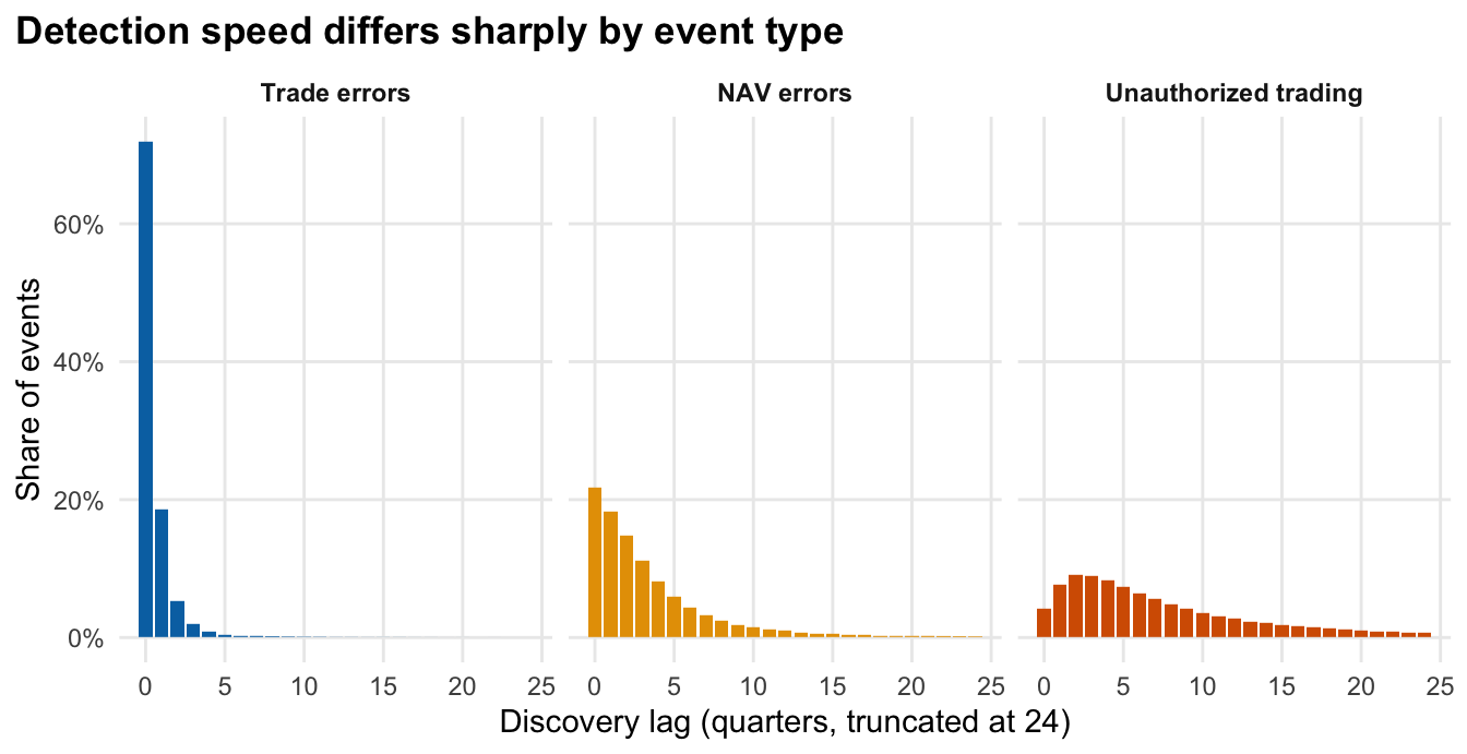
lags |>filter(lag <=24) |>count(type, lag) |>mutate(share = n /2e5, .by = type) |>mutate(type =factor(type, levels = type_lab)) |>ggplot(aes(lag, share, fill = type)) +geom_col(width =0.85) +facet_wrap(~type, nrow =1) +scale_fill_manual(values = type_col, guide ="none") +scale_y_continuous(labels = scales::label_percent()) +labs(x ="Discovery lag (quarters, truncated at 24)", y ="Share of events", title ="Detection speed differs sharply by event type") +theme_op()
Figure 1: Simulated share of events by discovery lag, per event type (200,000 draws each).
How to read the Discovery-Lag Distributions plot Each bar shows the share of events found a given number of quarters after they happened, so bars clustered at the left mean fast detection and a long spread to the right means slow detection.
What the plot tells you Detection speed differs sharply by event type. The median number of quarters to discovery is Trade errors: 0, NAV errors: 2, Unauthorized trading: 6, so trade errors are found almost at once while unauthorized trading often runs for years. The share of events discovered after the 40-quarter window is Trade errors 0.0%, NAV errors 0.1%, Unauthorized trading 2.7%, so few events fall outside the window, but for unauthorized trading they matter.
Loss grows while an event stays hidden, up to 4.2 times the initial size, and the measure here counts only loss that is still undiscovered. So the 2.7% of unauthorized-trading events beyond the window carry about 40% of the true undiscovered unauthorized-trading loss at the evaluation date (baseline, annual granularity, 200 databases).
This is why a standard method that looks only inside the 10-year history misses so much of that line.
Sanity check: size of the losses
An uncalibrated simulator can easily produce implausible losses, so we check the scale against an assumed AUM of $5.0B. Expected annual incurred loss (all events, discovered or not) over 200 simulated databases:
Code
sims <- parallel::mclapply(1:200, \(r) {simulate_database(base, rep = r) |>mutate(year =ceiling(origin /4)) |>summarise(inc =sum(severity), n =n(), .by =c(type, year))}, mc.cores =max(1L, parallel::detectCores() -2L)) |>bind_rows(.id ="rep")n_years <- params$horizon$n_origin /4by_type <- sims |>summarise(`Mean loss / yr`=sum(inc) / (n_distinct(rep) * n_years), `Events / yr`=sum(n) / (n_distinct(rep) * n_years), .by = type) |>mutate(Type = type_lab[type], `bps of AUM`=`Mean loss / yr`/ aum *1e4)# Single-year totals (all types), pooled over databases and origin years: the same basis as VaR on the Control Value page.year_totals <- sims |>summarise(inc =sum(inc), .by =c(rep, year))bind_rows( by_type |>select(Type, `Events / yr`, `Mean loss / yr`, `bps of AUM`),tibble(Type ="All types", `Events / yr`=sum(by_type$`Events / yr`), `Mean loss / yr`=mean(year_totals$inc), `bps of AUM`=mean(year_totals$inc) / aum *1e4)) |>mutate(Type =factor(Type, levels =c(type_lab, "All types"))) |>arrange(Type) |> gt::gt() |> gt::fmt_number(c(`Events / yr`, `bps of AUM`), decimals =1) |> gt::fmt_currency(`Mean loss / yr`, decimals =0) |> gt::tab_source_note(sprintf("Single-year total loss, pooled over %d databases x %d origin years: median %.1f bps, 95th percentile %.1f bps of AUM (VaR95 %s). Targeted range: 10-15 bps mean; this is an assumption, not a benchmark.",n_distinct(sims$rep), n_years, median(year_totals$inc) / aum *1e4, quantile(year_totals$inc, .95) / aum *1e4, fmt_usd(quantile(year_totals$inc, .95), 2)))
Table 2
Type
Events / yr
Mean loss / yr
bps of AUM
Trade errors
294.0
$1,262,567
2.5
NAV errors
29.2
$2,342,539
4.7
Unauthorized trading
1.4
$2,430,188
4.9
All types
324.6
$6,035,294
12.1
Single-year total loss, pooled over 200 databases x 10 origin years: median 8.6 bps, 95th percentile 23.0 bps of AUM (VaR95 $11.48M). Targeted range: 10-15 bps mean; this is an assumption, not a benchmark.
How to read the table Each row is an event type, showing how many events happen a year, the average yearly loss in dollars, and that loss as basis points (hundredths of a percent) of assets under management. The last row is the total for all types, and the note under the table shows how bad a single year can get.
What the table tells you Total expected loss is about $6.0M a year, or 12 bps of assets, inside the 10-15 bps target. Trade errors are most of the events but a small share of the dollars, unauthorized trading is about 1.4 events a year but roughly 40% of the loss, and a bad year (95th percentile) is about 23 bps, so the simulated firm is neither implausibly safe nor implausibly loss-making.
Sanity check table insights Total expected loss is about $6.0M a year, or 12 basis points of the assumed $5B in assets, which sits within the 10–15 bps target range. Trade errors make up nearly all of the roughly 325 events a year but only a fifth of the loss (2.5 of 12.1 bps), while the 1.4 unauthorized events a year are about 40% of it (4.9 bps), and a bad year (95th percentile) runs to about 23 bps, close to $11.5M.
One note on item 2: the “quarters” in the plot are discovery lags, while the “10-year window” is the horizon of the simulated loss history. If a board member might confuse the two, I’d say “10-year history” in place of “10-year window”.
Scenarios
Scenario
What changes
Baseline
Stable detection, proportional development
Heavy-tail shock
Two very large unauthorized-trading losses injected: $60M originating in quarter 12 and discovered in quarter 27 (reported), and $40M originating in quarter 20 and discovered in quarter 42 (after the evaluation date, so undiscovered)
Control improvement
Applies to all three event types. For every event whose discovery quarter \(d\) is after the change quarter \(c =\) 24, the discovery quarter becomes \(c + \lfloor (d - c)(1 - r) \rfloor\) with \(r =\) 50%. This covers both events already pending at \(c\) and events that originate afterwards. Severity is drawn before the shift, so only timing changes, not the loss amount.
Exposure growth
Volume growth rises to 3% per quarter
The two example controls on the Control Value page work differently from the control-improvement scenario above. They shift the lag-distribution parameters (additively, for the event types listed in params.yaml) for the whole simulated history before severities are drawn, so a faster-detected event is also smaller through the \((1 + e \times \text{lag})\) term.