Faster detection has value because (i) loss is recorded sooner, which improves information, and (ii) in this simulator an event’s size grows linearly with the time it stays undiscovered, through the factor \((1 + e \times \text{lag})\). Channel (ii) is the only way a control changes incurred loss; if \(e = 0\), mean and tail incurred loss are identical with and without the control, and only the information value in (i) remains. This page measures how much a detection control is worth under those assumptions. The effect sizes and costs are placeholders, not benchmarks; a real engagement would replace them with measured detection times and quoted prices.
Automated daily position/cash reconciliation against prime-broker statements
$400,000
Independent P&L verification
Independent P&L and limit-breach verification with prime-broker position feed
$700,000
How to read the table Each row is a detection control, with what it does and the annual cost assumed for it.
What the table tells you The two controls differ in scope and price: automated reconciliation costs $400K a year and mainly speeds up NAV and unauthorized-trading detection, while independent P&L verification costs $700K and also speeds up trade-error detection. The costs are placeholders, not quotes.
Each control shifts the lag distribution for some event types (see params.yaml). Baseline and control arms use the same seeds, so each pair of runs shares event counts and severity draws, and the saving is a paired difference.
Result: expected loss and tail
Code
base <- ctl |>filter(arm =="baseline")ctl |>transmute(Arm = ctl_lab[arm],`Mean incurred / yr`= mean_incurred_per_year,`bps of AUM`= mean_incurred_per_year / aum *1e4,`Saving / yr`=if_else(arm =="baseline", NA_real_, mean_saving_per_year),`Annual cost`= annual_cost,`Net / yr`= net_benefit_per_year,`Undiscovered at year 10`= mean_undiscovered,`95% VaR (annual)`= annual_var95,`95% ES (annual)`= annual_es95 ) |> gt::gt() |> gt::fmt_currency(-c(Arm, `bps of AUM`), decimals =2, suffixing =TRUE) |> gt::fmt_number(`bps of AUM`, decimals =1) |> gt::sub_missing(missing_text ="-") |> gt::tab_source_note("VaR/ES are over single origin-year totals pooled across 200 databases (2,000 years), so ES95 averages about 100 tail years. Savings are paired against the baseline arm. At full effectiveness the saving is also the most the control could cost and still break even.")
Table 2
Arm
Mean incurred / yr
bps of AUM
Saving / yr
Annual cost
Net / yr
Undiscovered at year 10
95% VaR (annual)
95% ES (annual)
Baseline
$6.04M
12.1
-
-
-
$12.62M
$11.48M
$31.79M
Reconciliation automation
$5.53M
11.1
$502.30K
$400.00K
$102.30K
$6.27M
$10.14M
$26.79M
Independent P&L verification
$5.30M
10.6
$735.12K
$700.00K
$35.12K
$4.54M
$9.44M
$23.37M
VaR/ES are over single origin-year totals pooled across 200 databases (2,000 years), so ES95 averages about 100 tail years. Savings are paired against the baseline arm. At full effectiveness the saving is also the most the control could cost and still break even.
How to read the table Each row is a scenario: no control, or one of the two controls. The table shows average loss per year, the saving against no control, the assumed cost, the net benefit, the loss still undiscovered at the end of year 10, and the loss in a bad year (VaR) and in the worst 5% of years (ES).
What the table tells you Both controls roughly pay for themselves on average loss alone, with net benefits of $102K and $35K a year. They also roughly halve the loss that has happened but is still unrecorded at the end of the history, from $12.6M to between $4.5M and $6.3M, and they lower loss in bad years.
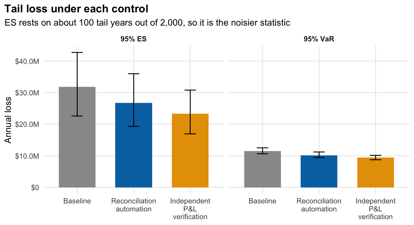
On expected loss alone, both controls are close to break-even: reconciliation automation saves $502.30K a year against a $400.00K cost (net $102.30K), and independent P&L verification saves $735.12K against $700.00K (net $35.12K). Put differently, the most each control could cost and still break even at full effectiveness is its mean saving. The simulated 95% expected shortfall of annual loss falls from $31.8M to $26.8M and $23.4M; the intervals below show how well that is pinned down. Because baseline and control share seeds, a paired bootstrap of the reduction is tighter than the separate intervals: ES95 falls by $5.0M (95% interval $3.0M to $7.4M) under reconciliation automation and by $8.4M ($5.1M to $12.2M) under independent P&L verification. Both the mean and the tail savings come from the same severity-growth mechanism (see the sensitivity below).
Code
bind_rows( tail_ci |>transmute(arm, stat ="95% VaR", value = var95, lo = var95_lo, hi = var95_hi), tail_ci |>transmute(arm, stat ="95% ES", value = es95, lo = es95_lo, hi = es95_hi)) |>mutate(arm =factor(arm, levels =names(ctl_lab))) |>ggplot(aes(arm, value, fill = arm)) +geom_col(width =0.65) +geom_errorbar(aes(ymin = lo, ymax = hi), width =0.2) +facet_wrap(~stat) +scale_fill_manual(values =c(baseline ="grey60", ctl_col), guide ="none") +scale_y_continuous(labels = fmt_usd) +scale_x_discrete(labels = \(x) str_wrap(ctl_lab[x], 14)) +labs(x =NULL, y ="Annual loss", title ="Tail loss under each control", subtitle ="ES rests on about 100 tail years out of 2,000, so it is the noisier statistic") +theme_op()
Figure 1: Pooled single-year loss. Error bars: 95% percentile bootstrap over the 200 databases.
How to read the plot Each pair of bars shows the loss in a bad year (the “95% VaR”: 1 year in 20 is worse) and the average loss in the worst 5% of years (the “95% ES”), with and without each control. The black whiskers show the uncertainty from using a finite number of simulated years.
What the plot tells you Both controls lower both tail measures, with independent P&L verification lowering them most. The whiskers overlap for the worst-years measure, so the exact size is uncertain, but comparing each control with the same simulated years shows the reduction is clearly above zero.
How effective must a control be? Break-even
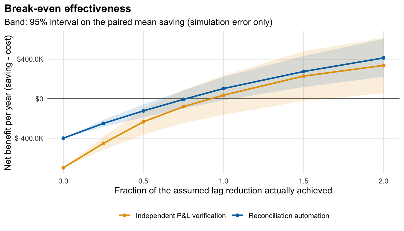
The size of the lag reduction is the least certain input. Scaling each control’s assumed shift by a factor (1 = as assumed, 0 = no effect) shows where the mean saving equals the annual cost.
Code
be <- res$beggplot(be$curve, aes(scale, net, colour = control)) +geom_hline(yintercept =0, colour ="grey40") +geom_ribbon(aes(ymin = net -1.96* se, ymax = net +1.96* se, fill = control), alpha =0.15, colour =NA) +geom_line(linewidth =0.9) +geom_point() +scale_colour_manual(values = ctl_col, labels = ctl_lab, name =NULL) +scale_fill_manual(values = ctl_col, guide ="none") +scale_y_continuous(labels = fmt_usd) +labs(x ="Fraction of the assumed lag reduction actually achieved", y ="Net benefit per year (saving - cost)", title ="Break-even effectiveness", subtitle ="Band: 95% interval on the paired mean saving (simulation error only)") +theme_op()
Figure 2
How to read the plot The horizontal axis is the share of the promised reduction in detection time that a control actually delivers (100% is as assumed). The vertical axis is net benefit per year, so the point where a line crosses zero is the break-even level, and the shaded band is simulation noise only.
What the plot tells you Reconciliation automation must deliver about 77% of its promised improvement to pay for itself, and independent P&L verification about 92%. The second is far less forgiving: it has little margin for the control to under-deliver.
How to read the table The table restates the break-even points from the plot as percentages, and adds the most each control could cost and still pay for itself if it works exactly as promised.
What the table tells you The cheaper control has more slack both ways: it can under-deliver more, and the assumed cost sits well below its break-even cost. The independent P&L control is close to its limit on both measures.
The band reflects Monte Carlo error only. It does not include uncertainty in the cost, the lag shift, or the severity-growth assumption, which are likely larger.
Sensitivity to severity growth
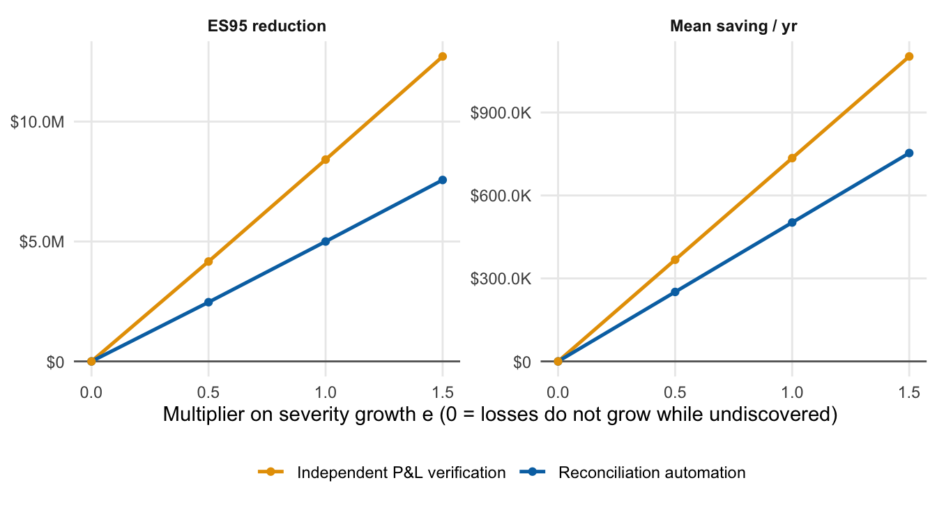
Every dollar saving on this page flows through the severity-growth parameter \(e\). The study was re-run with \(e\) multiplied by 0, 0.5, 1 (as assumed) and 1.5, using the same seeds.
Code
base_es <- sens |>filter(arm =="baseline") |>select(e_mult, base_es = annual_es95)sens |>filter(arm !="baseline") |>left_join(base_es, by ="e_mult") |>transmute(e_mult, Control = ctl_lab[arm], `Mean saving / yr`= mean_saving_per_year, `ES95 reduction`= base_es - annual_es95) |>pivot_longer(c(`Mean saving / yr`, `ES95 reduction`), names_to ="Measure") |>ggplot(aes(e_mult, value, colour = Control)) +geom_hline(yintercept =0, colour ="grey40") +geom_line(linewidth =0.9) +geom_point() +facet_wrap(~Measure, scales ="free_y") +scale_colour_manual(values =setNames(ctl_col, ctl_lab[names(ctl_col)]), name =NULL) +scale_y_continuous(labels = fmt_usd) +labs(x ="Multiplier on severity growth e (0 = losses do not grow while undiscovered)", y =NULL) +theme_op()
Figure 3: Paired mean saving and ES95 reduction against the multiplier on severity growth e (1 = as assumed).
How to read the plot The horizontal axis scales how quickly loss grows while an event stays hidden (1 is the assumption used everywhere else, 0 means loss does not grow at all). The vertical axes show the yearly saving (left) and the reduction in worst-year loss (right) for each control.
What the plot tells you The dollar value of both controls depends entirely on this one assumption: with no growth the savings are zero, and at half the assumed growth $251K a year does not cover reconciliation automation’s cost. A firm should measure how much its own losses grow while undiscovered before relying on the dollar figures.
Code
s0 <- sens |>filter(e_mult ==0, arm !="baseline")
With \(e = 0\) the paired saving is $0 to $0 a year: any value that is not exactly zero is a simulation artefact (paired runs share event counts and severities, so with \(e = 0\) incurred loss should be identical). The tail reduction vanishes in the same way.
Information value
The cleanest benefit that does not depend on severity growth is earlier information. At the evaluation date, the loss that has already happened but is not yet in the database falls from $12.6M to $6.3M under reconciliation automation and $4.5M under independent P&L verification. A smaller undiscovered balance means the reported loss trend is closer to the true one, and the loss data a firm uses for capital, board reporting or allocator disclosure is less incomplete. This benefit is not converted to dollars here, because its value depends on how the firm uses the data.
Caveats specific to this page
Incurred loss changes under a control only through the severity-growth term \((1 + e \times \text{lag})\). If losses do not grow while undiscovered (\(e = 0\)), neither the mean nor the tail of incurred loss changes; the only benefit left is earlier information, shown above as undiscovered loss at year 10.
Control cost is a single annual figure with no ramp-up, no false-positive workload and no risk of the control failing.
Losses are gross. Loss-event insurance, recoveries from counterparties and compensation that is later clawed back would reduce net losses and therefore net savings.
No discounting, no correlation with market stress, and no regulatory or reputational effects are modelled.