Misreading the Attacker – Where Will the Attacker Strike?

Why the textbook answer is fragile

The textbook equilibrium works by making the crew exactly indifferent across 5 targets. That razor’s edge is what makes the plan efficient, and also what makes it brittle: when the crew’s real payoffs differ from our estimates, the crew steps off the edge toward the target we left weakest.

Misjudged payoffs

We drew 3,000 versions of the crew. In each, every success payoff is multiplied by a random error (lognormal, sigma = 0.35). Every strategy faces the same draws.

Code

ord <- ms$strategy[order(ms$mean)]
hits <- draws |>
  summarise(n = n(), loss = first(loss), .by = c(strategy, target)) |>
  mutate(share = n / sum(n), .by = strategy) |>
  mutate(strategy = factor(strategy, levels = rev(ord)),
         asset = factor(ASSET_SHORT[target], levels = ASSET_SHORT)) |>
  arrange(strategy, asset) |>
  mutate(xmid = cumsum(share) - share / 2, .by = strategy)
callout <- hits |> filter(target == "PIPE", share >= 0.03)   # rare but costly hits

share_of <- \(s, a) sum(hits$share[hits$strategy == s & hits$target == a])
rb_corp  <- share_of("robust", "CORP")
tb_pipe  <- share_of("textbook", "PIPE")

ggplot(hits, aes(x = share, y = strategy, fill = asset)) +
  geom_col(width = 0.7, color = "white", linewidth = 0.3,
           position = position_stack(reverse = TRUE)) +
  geom_text(aes(label = ifelse(share >= 0.08, fmt_m(loss), "")),
            position = position_stack(vjust = 0.5, reverse = TRUE), size = 3, color = "white") +
  geom_text(data = callout, aes(x = xmid, y = strategy, label = fmt_m(loss)),
            inherit.aes = FALSE, nudge_y = 0.48, size = 3, color = "#2E7D6B", fontface = "bold") +
  scale_x_continuous(labels = scales::percent, expand = expansion(mult = c(0, 0.01))) +
  scale_y_discrete(labels = STRAT_LABELS) +
  scale_fill_manual(values = ASSET_COLS, name = NULL, drop = FALSE) +
  guides(fill = guide_legend(nrow = 1)) +
  labs(x = "Share of simulated crews", y = NULL,
       title = "Where the crew strikes when we misjudge it",
       subtitle = "Labels show our loss if that asset is hit") +
  theme(legend.position = "top", panel.grid.major.y = element_blank())

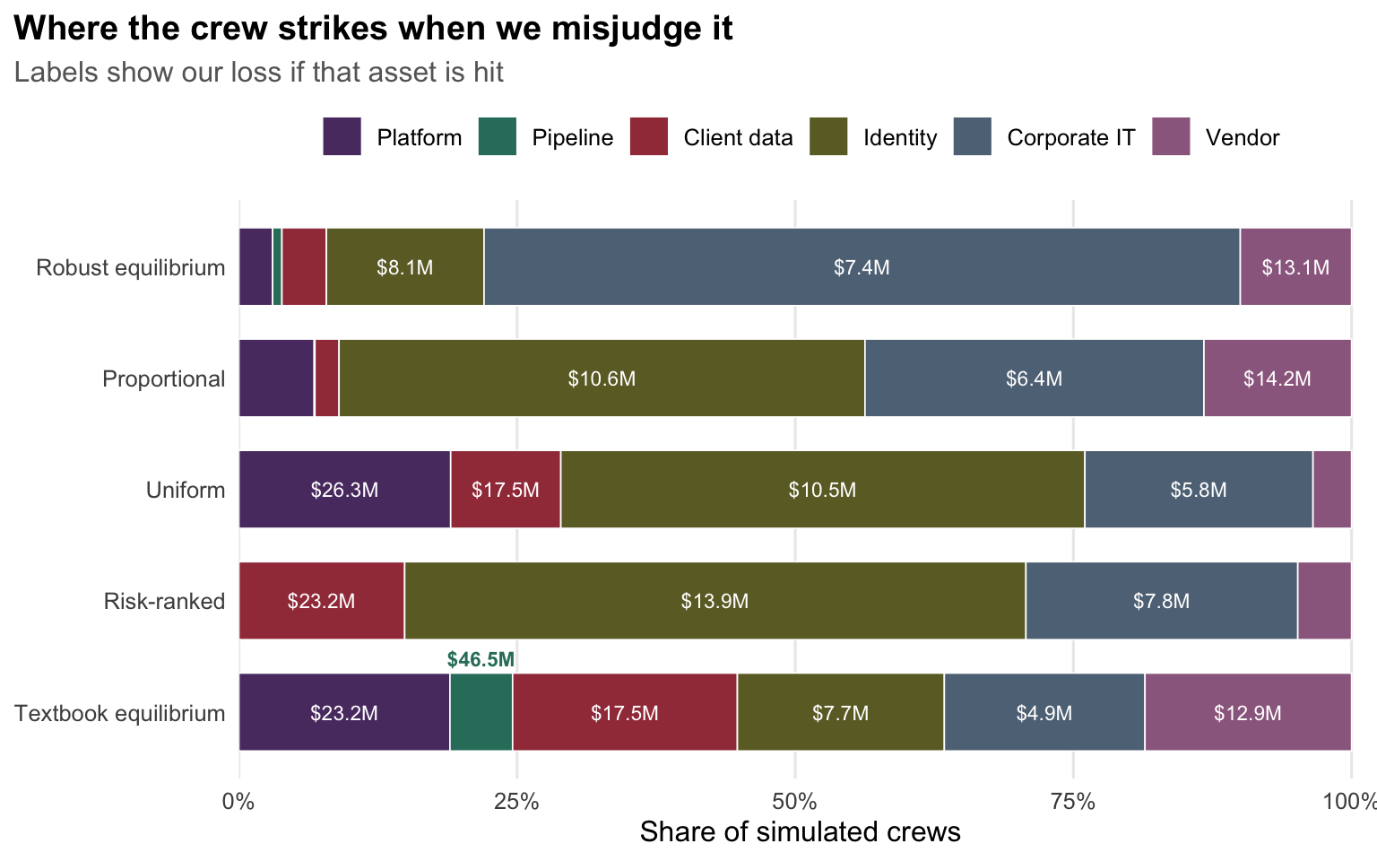
Stacked horizontal bars, one per strategy, showing the share of simulated crews attacking each of six assets. Under the robust strategy about two-thirds of crews hit corporate IT at a loss of 7.4 million dollars. Under the textbook strategy crews spread across all six assets, including the pipeline at 46.5 million dollars. — Figure 1: Where simulated crews strike under each strategy when their payoffs differ from our estimate. Labels show our loss if that asset is hit.

How to read the plot. Each bar is one strategy, ordered from lowest average loss (top) to highest. The colored segments show the share of simulated crews that attack each asset, and the label is what that attack would cost us.

What the plot tells you. Robust funnels 68% of crews onto corporate IT, a cheap hit. The textbook plan scatters them across all six assets, and about one crew in 18 reaches the pipeline, a $46.5M loss.

Code

ms |>
  arrange(mean) |>
  transmute(Strategy = STRAT_LABELS[strategy], mean, p50, p95, p99,
            Hit = sprintf("%s (%s)", ASSET_SHORT[top_target], fmt_pct(top_share))) |>
  gt() |>
  cols_label(mean = "Mean", p50 = "Median", p95 = "95th pct.", p99 = "99th pct.", Hit = "Most-hit asset") |>
  tab_spanner("Loss ($M)", columns = c(mean, p50, p95, p99)) |>
  fmt_number(columns = c(mean, p50, p95, p99), decimals = 1) |>
  gt_se()

Table 1: Loss statistics when the crew’s payoffs are misjudged, by strategy.

Strategy	Loss ($M)				Most-hit asset
Strategy	Mean	Median	95th pct.	99th pct.	Most-hit asset
Robust equilibrium	9.0	7.4	14.9	19.4	Corporate IT (68%)
Proportional	10.7	10.6	22.3	22.3	Identity (47%)
Uniform	13.3	10.5	26.3	26.3	Identity (47%)
Risk-ranked	13.9	13.9	23.2	23.2	Identity (56%)
Textbook equilibrium	15.3	12.9	46.5	46.5	Client data (20%)

How to read the table. Each row is a strategy, sorted by average loss. The loss columns show the average, the middle case, and the bad cases that 1 in 20 and 1 in 100 simulated crews exceed. The last column shows the asset attacked most often and the share of crews that attack it.

What the table tells you. The robust strategy has the lowest average and the smallest bad cases. The textbook equilibrium has the worst average, and its 95th percentile is 3.1 times the robust figure. The crew’s favorite target also differs across strategies.

How much each strategy relies on a perfect read

If our read of the crew is wrong, the robust strategy loses $1.6M more than planned, and the textbook strategy loses $10.3M more. The textbook plan’s efficiency rests almost entirely on accurate intelligence.

The robust equilibrium

The robust strategy assumes the crew mostly, but not always, picks the best target. It gives each target a chance of being hit that rises with how attractive it is to the crew, then minimizes our expected loss against those chances. A rationality parameter, $\lambda$, controls how sharp the crew is.

We set $\lambda =$ 2, chosen on a separate set of simulated crews so the choice is not tuned to the results we report. Optimizing at 2 gives the lowest average loss: $9.13M at 1, $9.03M at 2, $9.83M at 3 and $11.21M at 5.

The math behind the equilibrium

The crew attacks target $t$ with probability

\[q_t(c) = \frac{\exp(\lambda U_a(t,c))}{\sum_s \exp(\lambda U_a(s,c))}.\]

We minimize $f(c) = \sum_t q_t(c)\,\ell_t(c)$ over feasible coverage, with $\ell_t$ our loss on target $t$. The gradient is analytic and checked against finite differences. A multistart SLSQP search handles the nonconvexity.

Noisy attackers

Code

sweep |>
  mutate(strategy = factor(strategy, levels = STRAT_ORDER)) |>
  ggplot(aes(lambda, expected_loss, color = strategy, linetype = strategy)) +
  geom_line(linewidth = 1) +
  geom_point(size = 1.8) +
  scale_x_log10(breaks = LAMBDA_GRID, labels = LAMBDA_GRID) +
  scale_color_manual(values = STRAT_COLS, labels = STRAT_LABELS, name = NULL) +
  scale_linetype_manual(values = STRAT_LTY, labels = STRAT_LABELS, name = NULL) +
  scale_y_continuous(labels = scales::label_dollar(suffix = "M")) +
  labs(x = "Crew sharpness (lambda, log scale)", y = "Expected loss",
       title = "Robust wins unless the crew is nearly random") +
  guides(color = guide_legend(nrow = 2))

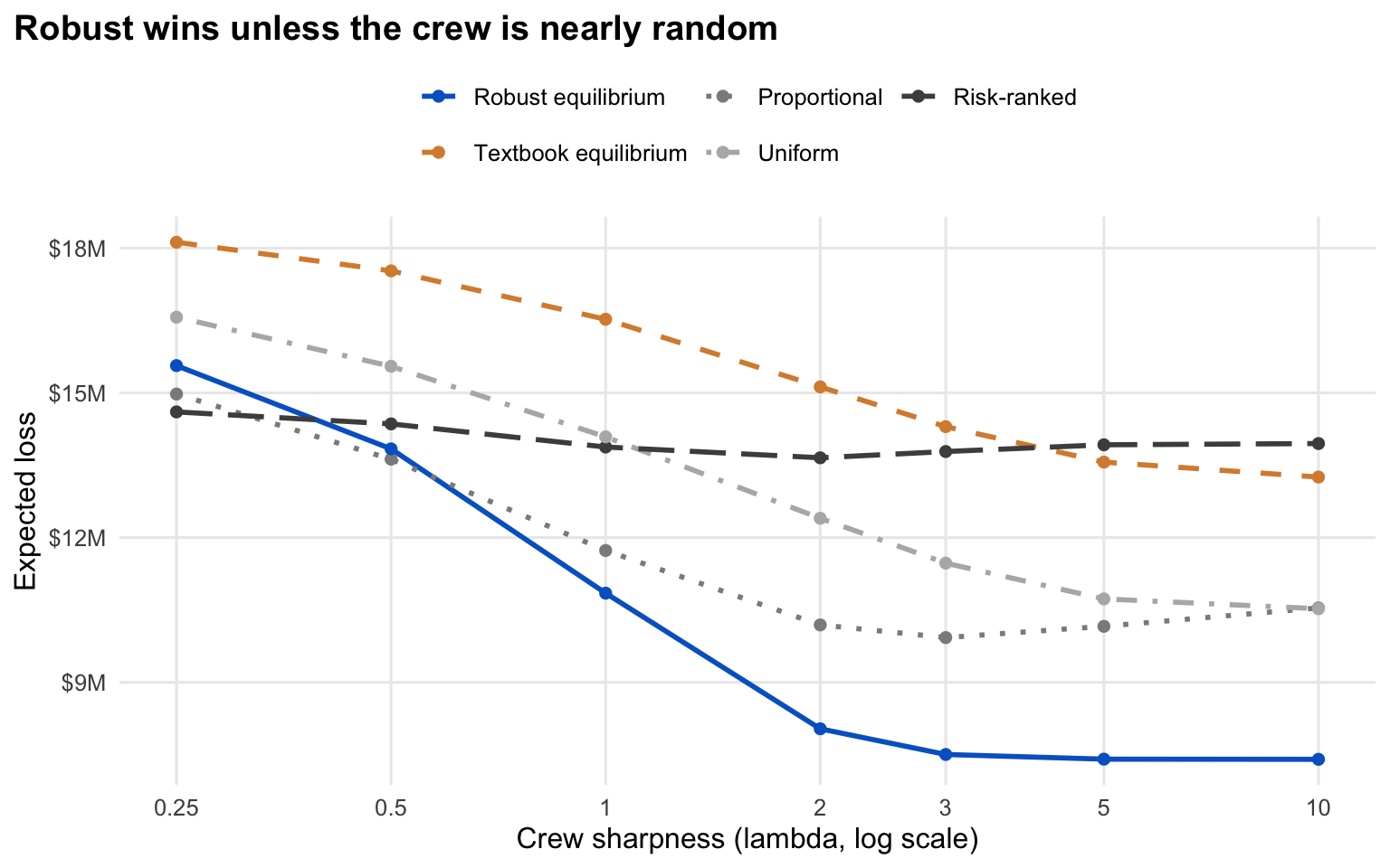
Line chart of expected loss against lambda on a log axis for five strategies. The robust strategy is lowest from lambda of 1 upward. The textbook equilibrium is highest at the lower values. — Figure 2: Expected loss against a noisy crew as the crew becomes sharper (higher lambda). Strategies are held fixed.

How to read the plot. The horizontal axis shows how sharp the crew is: low values mean it picks targets almost at random, high values mean it always picks its best one. Each line is a strategy whose coverage is fixed. The vertical axis is our expected loss.

What the plot tells you. The robust strategy has the lowest loss once the crew is moderately sharp (2 is our base case; robust leads from 1 upward). For a nearly random crew, simpler plans do slightly better. The textbook equilibrium is worse than robust at every sharpness.

The budget frontier

Code

fr |>
  mutate(strategy = factor(strategy, levels = STRAT_ORDER)) |>
  ggplot(aes(budget, mc_mean, color = strategy, linetype = strategy)) +
  geom_vline(xintercept = BUDGET_BASE, color = "gray60", linetype = "dotted") +
  geom_line(linewidth = 1) +
  scale_color_manual(values = STRAT_COLS, labels = STRAT_LABELS, name = NULL) +
  scale_linetype_manual(values = STRAT_LTY, labels = STRAT_LABELS, name = NULL) +
  scale_x_continuous(labels = scales::label_dollar(suffix = "M")) +
  scale_y_continuous(labels = scales::label_dollar(suffix = "M")) +
  labs(x = "Allocable budget", y = "Expected loss if we misjudge the crew",
       title = "Robust stays ahead as the budget grows") +
  guides(color = guide_legend(nrow = 2))

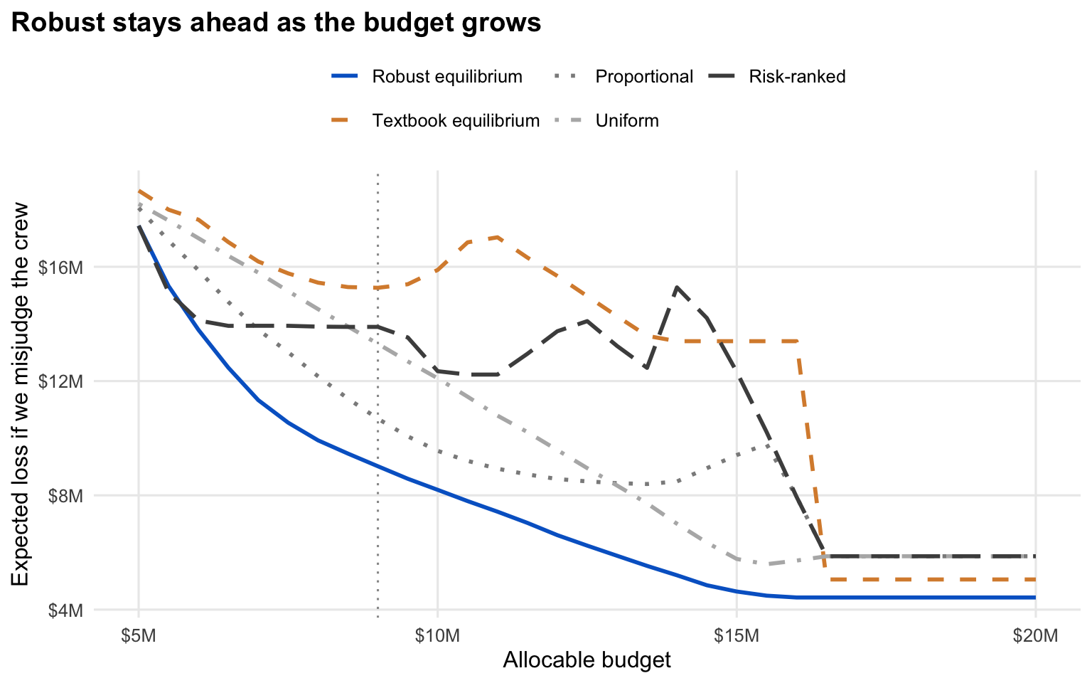
Line chart of mean loss against budget from 5 to 20 million dollars for five strategies. The robust strategy lies lowest or tied at nearly every budget. A vertical line marks the 9 million dollar base budget. — Figure 3: Expected loss when we misjudge the crew, by budget. The vertical line marks the base budget.

How to read the plot. Each line shows average loss by budget for one strategy when we misjudge the crew. The dotted line is our base budget.

What the plot tells you. Robust is lowest at nearly every budget. Extra money can hurt a simple plan: risk-ranked rises from $12.2M at $11.0M to $15.3M at $14.0M, and textbook from $15.3M at $9.0M to $17.0M at $11.0M, as new coverage pushes the crew toward a thin asset. At $5.5M a baseline edges ahead, though robust still beats the sharp crew it is built for. Above $16.5M every asset hits its cap.

Moving from $9.0M to $10.0M lowers the expected loss from misjudging the crew by $0.83M under robust and $1.55M under risk-ranked. Robust still leads at $10.0M: $8.2M against $12.3M. Across the budget grid from $5.0M to $20M, robust is lowest or tied at every budget except $5.5M.

Try it: move the slider to see how coverage and the crew’s likely target change.

Code

html`<div class="slider-sentence">At <b>$${budget.toFixed(1)}M</b>, the crew's best target is <b>${rr.target_label}</b> under risk-ranked and <b>${rb.target_label}</b> under robust. Expected loss if we misjudge the crew: <b>$${rr.mc_mean.toFixed(1)}M</b> against <b>$${rb.mc_mean.toFixed(1)}M</b>.</div>`

How to read the plot. Drag the slider to choose a budget. Each group of bars is an asset, with the gray bar for risk-ranked coverage and the blue bar for the robust strategy. The sentence under the chart states the crew’s likely target and our expected loss under each approach.

What the plot tells you. As the budget changes, risk-ranked keeps funding the same few assets, while the robust strategy spreads protection toward the places a crew is likely to hit. The sentence shows what that difference costs us.