Allocating the Budget

Where Will the Attacker Strike? Four ways to split a security budget

All money is in $M. Losses are expected loss per targeted ransomware campaign, and the model assumes one campaign per year. All values are illustrative.

The firm

The firm has 500 staff. Its cloud platform is critical infrastructure for its bank and broker clients. It has $9.0M a year to allocate across six assets. That budget includes a hygiene floor: every asset keeps at least 25% coverage, because compliance demands it.

Code

mu <- log(assets$L) - LOSS_SIGMA^2 / 2
assets |>
  mutate(
    Asset = ASSET_SHORT[asset_id],
    median = exp(mu),
    lo = exp(mu - 1.645 * LOSS_SIGMA),
    hi = exp(mu + 1.645 * LOSS_SIGMA),
    ci = sprintf("%.1f to %.1f", lo, hi)
  ) |>
  select(Asset, L, median, ci, V, k, c_max, p_heat) |>
  gt() |>
  tab_spanner("Defender loss ($M)", columns = c(L, median, ci)) |>
  cols_label(L = "Mean", median = "Median", ci = "90% interval", V = "Crew value ($M)",
             k = "Cost to cover ($M)", c_max = "Coverage cap", p_heat = "Heat-map likelihood") |>
  fmt_number(columns = c(L, median, V, k), decimals = 1) |>
  fmt_number(columns = c(c_max, p_heat), decimals = 2) |>
  tab_source_note("Illustrative values. Loss is treated as the mean of a lognormal with sigma = 0.8; median and interval are shown for context only.") |>
  gt_se()

Table 1: The six assets and their parameters. Illustrative values.

Asset	Defender loss ($M)			Crew value ($M)	Cost to cover ($M)	Coverage cap	Heat-map likelihood
Asset	Mean	Median	90% interval	Crew value ($M)	Cost to cover ($M)	Coverage cap	Heat-map likelihood
Platform	45.0	32.7	8.8 to 121.8	6.0	4.0	0.90	0.30
Pipeline	60.0	43.6	11.7 to 162.4	2.5	3.0	0.90	0.15
Client data	30.0	21.8	5.8 to 81.2	5.0	2.5	0.90	0.30
Identity	18.0	13.1	3.5 to 48.7	7.0	2.0	0.90	0.25
Corporate IT	10.0	7.3	1.9 to 27.1	5.5	3.0	0.85	0.50
Vendor	20.0	14.5	3.9 to 54.1	4.0	5.0	0.70	0.20
Illustrative values. Loss is treated as the mean of a lognormal with sigma = 0.8; median and interval are shown for context only.

How to read the table. Each row is an asset. The first block is what a successful attack costs us; “crew value” is what the crew gains. “Cost to cover” is the price of full coverage, and the cap is the most protection we can reach.

What the table tells you. Our biggest loss (the pipeline) is among the crew’s least valued targets, while identity is the crew’s favorite and costs us far less. The wide 90% intervals warn that a typical loss can differ greatly from the average.

Where we and the crew disagree

Code

assets |>
  mutate(rank_L = rank(L), rank_V = rank(V), label = ASSET_SHORT[asset_id]) |>
  ggplot(aes(rank_L, rank_V)) +
  geom_abline(slope = 1, intercept = 0, linetype = "dashed", color = "gray50") +
  geom_point(size = 3.5, color = "#0166CC") +
  ggrepel::geom_text_repel(aes(label = label), size = 4, box.padding = 0.5) +
  scale_x_continuous(breaks = 1:6, limits = c(0.7, 6.3)) +
  scale_y_continuous(breaks = 1:6, limits = c(0.7, 6.3)) +
  labs(x = "Rank by our loss (6 = largest)", y = "Rank by crew value (6 = most attractive)",
       title = "Our biggest worries are not the crew's favorites")

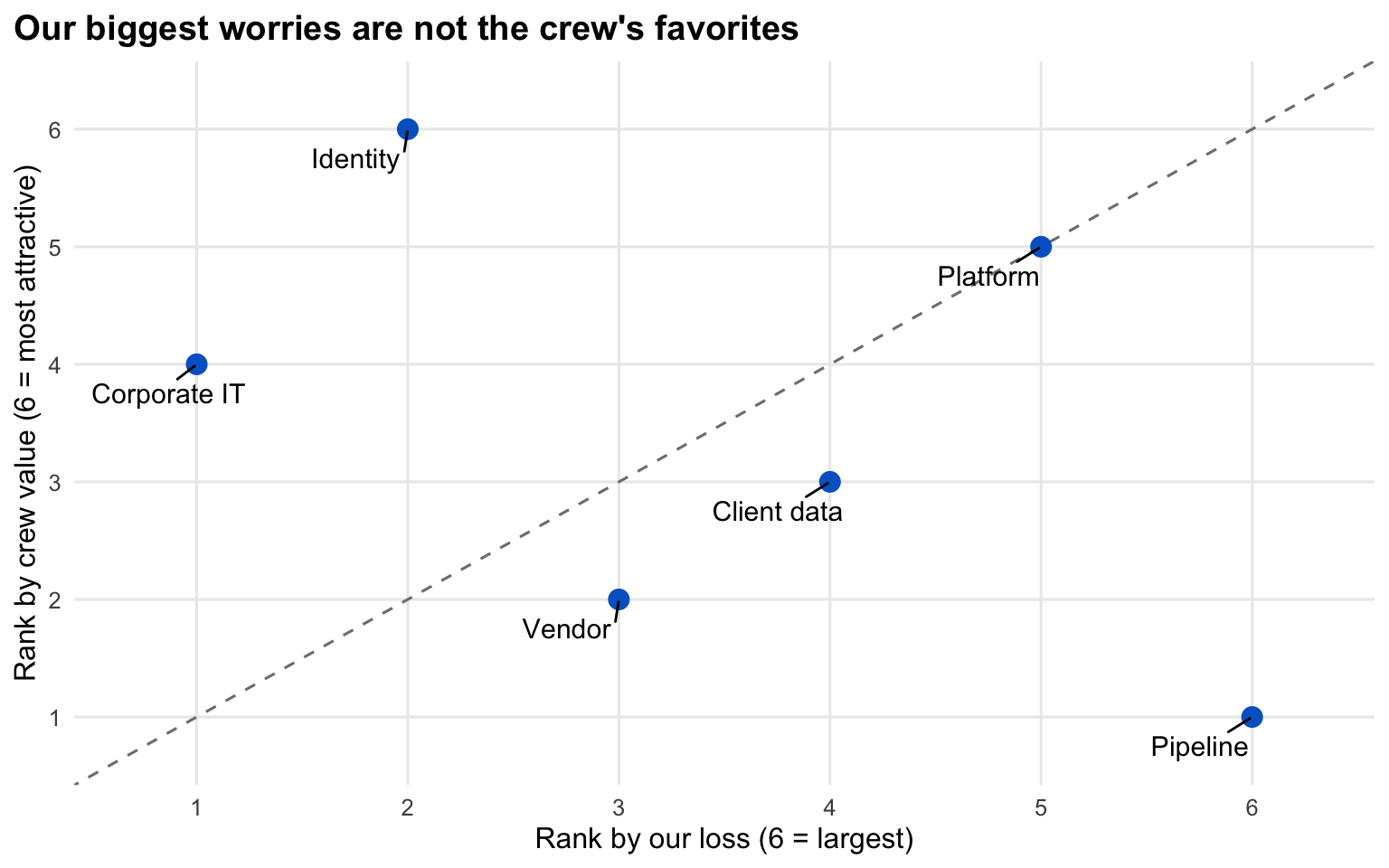
Scatter plot of six assets by rank of defender loss on the horizontal axis and rank of crew value on the vertical axis, with a diagonal reference line. Pipeline and identity lie far from the line; platform lies on it. — Figure 1: Rank of each asset by our loss against rank by the crew’s value. Distance from the diagonal measures disagreement.

How to read the plot. Each dot is an asset. Moving right means a larger loss for us; moving up means more attractive to the crew. The dashed diagonal marks assets where both sides agree on the ranking.

What the plot tells you. The pipeline is our largest loss but ranks last for the crew, so the crew has little reason to attack it. Identity is the reverse. A plan built only on our own risk ranking will misjudge where the crew goes.

Four strategies at the base budget

We compare four ways to spend $9.0M. The robust strategy joins on page 4.

Code

four <- c("risk_ranked", "proportional", "uniform", "textbook")
base$strategies |>
  filter(strategy %in% four) |>
  left_join(sm |> select(strategy, target), by = "strategy") |>
  mutate(
    strategy = factor(STRAT_LABELS[strategy], levels = STRAT_LABELS[four]),
    asset = factor(ASSET_SHORT[asset_id], levels = ASSET_SHORT),
    hit = ifelse(asset_id == target, "Crew's target", "Other asset")
  ) |>
  ggplot(aes(asset, coverage, fill = hit)) +
  geom_col(width = 0.75) +
  facet_wrap(~strategy, ncol = 2) +
  scale_fill_manual(values = c("Crew's target" = "#7A3E9D", "Other asset" = "#C8C8C8"), name = NULL) +
  scale_y_continuous(labels = scales::percent, limits = c(0, 1)) +
  labs(x = NULL, y = "Coverage") +
  theme(axis.text.x = element_text(angle = 30, hjust = 1))

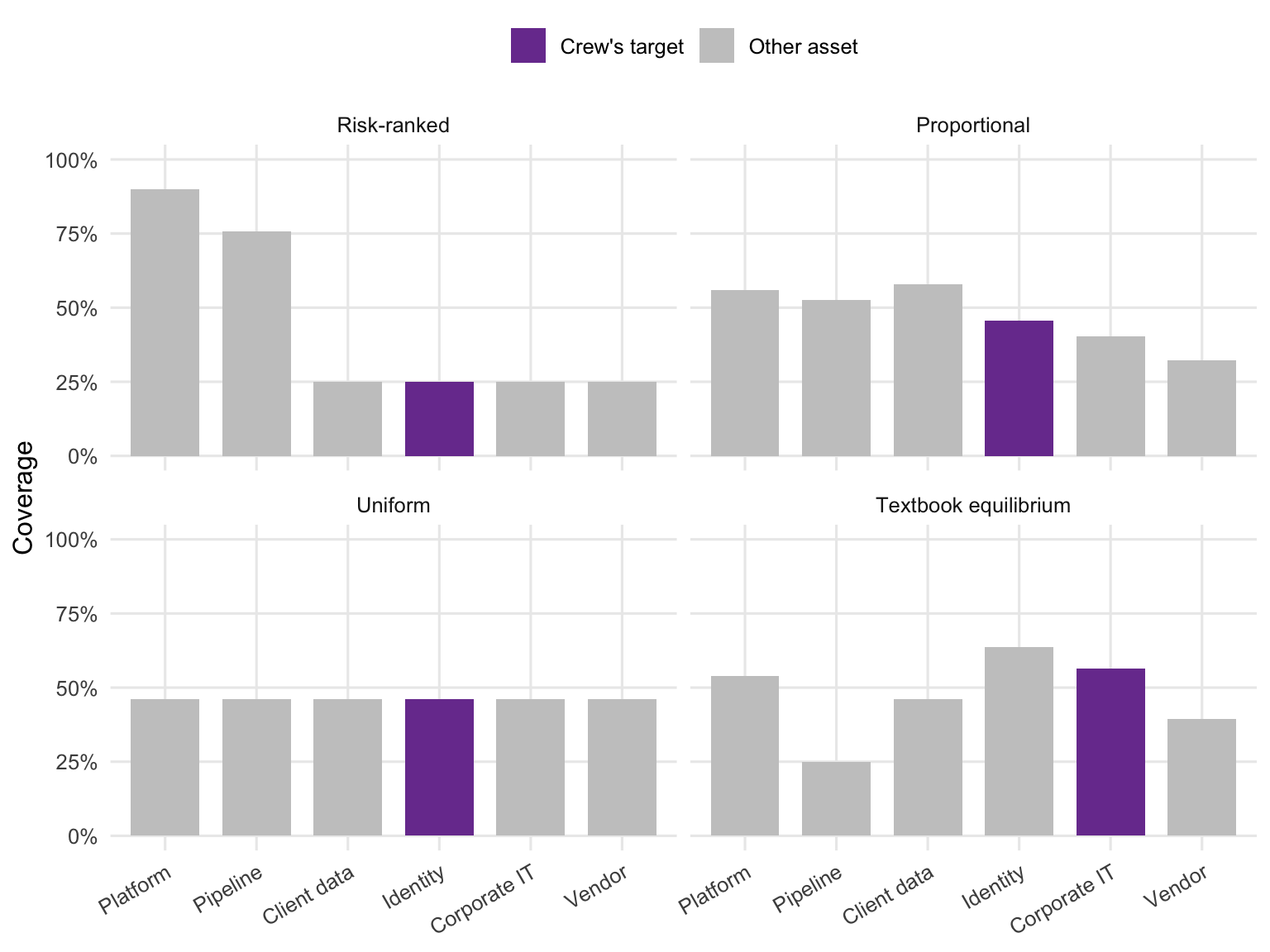
Four bar-chart panels, one per strategy, showing coverage on each of six assets. The attacked asset is highlighted: identity for risk-ranked, proportional and uniform, and corporate IT for the textbook equilibrium. — Figure 2: Coverage by asset under four strategies. The crew’s chosen target is highlighted in each panel.

How to read the plot. Each panel is one way to split the budget. Bars show how much of each asset is protected. The purple bar is the asset the crew would attack if it reads our defenses perfectly.

What the plot tells you. Risk-ranked piles protection onto two assets and leaves identity at the floor, which is where the crew goes. Proportional and uniform spread money out but still leave identity as the best target. Only the textbook plan changes the crew’s destination.

Code

sm |>
  filter(strategy %in% four) |>
  transmute(Strategy = STRAT_LABELS[strategy], Target = ASSET_SHORT[target], Loss = loss_rational) |>
  gt() |>
  cols_label(Target = "Crew target", Loss = "Expected loss ($M)") |>
  fmt_number(columns = Loss, decimals = 1) |>
  gt_se()

Table 2: Crew target and our expected loss under each strategy, assuming a perfectly rational crew.

Strategy	Crew target	Expected loss ($M)
Risk-ranked	Identity	13.9
Proportional	Identity	10.6
Uniform	Identity	10.5
Textbook equilibrium	Corporate IT	4.9

How to read the table. Each row is a strategy. The second column is the asset the crew attacks if it picks its best option. The third is our average loss from that attack.

What the table tells you. Risk-ranking has the highest loss. The textbook plan looks far better, but this table assumes we know exactly what the crew wants. Page 4 tests that assumption.

Interpretation

Risk-ranked funds the platform and pipeline and leaves identity at the floor. The crew sees this and goes to identity, for an expected loss of $13.9M.

The textbook equilibrium does something cleverer. It sets coverage so that the crew earns the same on 5 of the six assets. It lets the attack fall on corporate IT, a low-impact target, and cuts expected loss to $4.9M.

The trick has a price. The crew values the pipeline too little to bother, so the textbook plan holds the pipeline at 25%, the floor. The pipeline is our largest single loss.

This is the trap: the plan only works if we’ve read the crew perfectly.

Alignment check

What if the crew wanted what we fear most? We reran the comparison with crew values proportional to our losses. The textbook plan then costs $13.5M, with the crew attacking identity systems. Risk-ranked costs $23.2M, with the crew attacking client data.

The gap does not close. Concentration itself is the problem, not just misreading the attacker: risk-ranked spends heavily on a few assets and leaves the rest cheap to hit, whatever the crew wants.