---
title: "Decision Map & Reputation"
subtitle: "Where the pay line sits, and what each choice teaches the crew"
---
```{r setup}
#| include: false
source("R/00_params.R"); source("R/01_utils.R"); source("R/90_theme.R")
library(dplyr); library(ggplot2); library(gt)
wa <- read_result("walkaway")
rep <- read_result("reputation")
grid <- rep$grid
p0b <- P$reputation$p0_base
at_p0 <- \(p) grid |> filter(abs(p0 - p) < 1e-9)
cost_at <- \(p, f, pol) at_p0(p) |> filter(firm == f, policy == pol) |> pull(cost_10y)
att_at <- \(p, f, pol) at_p0(p) |> filter(firm == f, policy == pol) |> pull(attacks_10y)
saving <- \(p, f) cost_at(p, f, "rational") - cost_at(p, f, "never")
fragile_cross <- grid |>
filter(firm == "fragile") |>
summarise(gap = cost_10y[policy == "rational"] - cost_10y[policy == "never"], .by = p0) |>
filter(gap > 0) |> slice_min(p0, n = 1) |> pull(p0)
prof <- wa$profiles
fr <- prof |> filter(profile == "fragile")
dv <- rep$deviation
pv_of <- \(e, f, pol) dv$cost_10y_pv[dv$eta == e & dv$firm == f & dv$policy == pol]
eta_b <- P$reputation$eta_base
be <- rep$break_even
be_of <- \(f) be$eta_star[be$firm == f]
ojs_define(base_params = as.data.frame(BASE), rep_grid = rep$grid |> select(p0, firm, policy, cost_10y, attacks_10y))
```
*All money is in $M and all values are illustrative.*
## The decision map
The map below puts the board's two unknowns on one picture: how long a restore would take (across) and what the crew demands (up). Below the line, paying is cheaper than restoring; above it, we should refuse. Move the slider to see how much the line depends on trust in our backups. The map describes the day-one choice, before any restore has been tried.
```{ojs}
//| echo: false
//| output: false
import {walkAway, neverPayRestore} from "./assets/js/walkaway.js"
base = transpose(base_params)[0]
```
```{ojs}
//| echo: false
viewof bcred = Inputs.range([0.5, 0.99], {step: 0.01, value: 0.80, label: "Backup credibility"})
```
```{ojs}
//| echo: false
//| output: false
mapData = d3.range(1, 30.001, 0.25).map(t => ({
  T: t,
  R: walkAway({...base, T_r: t, b: bcred}),
  Rbase: walkAway({...base, T_r: t, b: 0.8})
}))
clamp = v => Math.max(0, Math.min(8, v))
```
```{ojs}
//| echo: false
//| label: fig-map
//| fig-cap: "Decision map at the selected backup credibility. Amber: paying is cheaper. Blue: restoring is cheaper. Dashed gray: the boundary at the base credibility of 0.80."
Plot.plot({
  height: 430, marginLeft: 60, marginBottom: 45, marginRight: 20,
  style: {fontFamily: "inherit", fontSize: "13px"},
  x: {domain: [1, 30], label: "Restore time from backups (days)", labelAnchor: "center", ticks: [1, 5, 10, 15, 20, 25, 30]},
  y: {domain: [0, 8], label: "Ransom demand", tickFormat: d => "$" + d + "M"},
  marks: [
    Plot.areaY(mapData, {x: "T", y1: 0, y2: d => clamp(d.R), fill: "#F2C46D", fillOpacity: 0.35}),
    Plot.areaY(mapData, {x: "T", y1: d => clamp(d.R), y2: 8, fill: "#0166CC", fillOpacity: 0.15}),
    Plot.line(mapData, {x: "T", y: "Rbase", stroke: "#9A9A9A", strokeDasharray: "6,4", strokeWidth: 1.5, clip: true}),
    Plot.line(mapData, {x: "T", y: "R", stroke: "#3A3A3A", strokeWidth: 2.5, clip: true,
      channels: {"Walk-away ($M)": d => d.R.toFixed(2)}, tip: true}),
    Plot.text([{x: 28.5, y: 0.5}], {x: "x", y: "y", text: () => "Pay", textAnchor: "end", fontWeight: "bold", fill: "#7a5a12", fontSize: 15}),
    Plot.text([{x: 2, y: 7.4}], {x: "x", y: "y", text: () => "Don't pay", textAnchor: "start", fontWeight: "bold", fill: "#0166CC", fontSize: 15}),
    Plot.dot([{T: 10, D: 2.5}], {x: "T", y: "D", r: 6, fill: "#0b0b0b", stroke: "white", strokeWidth: 2}),
    Plot.text([{T: 10, D: 2.5}], {x: "T", y: "D", text: () => "Our firm today", dx: 10, dy: 14, textAnchor: "start", fontWeight: "bold"})
  ]
})
```
```{ojs}
//| echo: false
r10 = walkAway({...base, T_r: 10, b: bcred})
t0 = neverPayRestore({...base, b: bcred})
r1 = walkAway({...base, T_r: 1, b: bcred})
html`<div class="slider-sentence">With backup credibility of <b>${bcred.toFixed(2)}</b>, at a 10-day restore we would pay any demand up to <b>$${r10.toFixed(2)}M</b>. ${t0 > 1
  ? html`Below <b>${t0.toFixed(1)} days</b> of restore time, we would not pay at any price.`
  : html`Even with a 1-day restore, paying up to <b>$${r1.toFixed(2)}M</b> would still be rational, because a failed restore would take so long.`}</div>`
```
```{=html}
<noscript>
```
```{r}
#| echo: false
#| fig-alt: "Static decision map at backup credibility 0.80: the pay region lies below a rising boundary line that crosses zero near 2.3 days of restore time and reaches about 2.4 million dollars at 10 days."
#| fig-height: 5
decision_map(wa$boundaries, 0.8) +
geom_line(data = filter(wa$boundaries, b == 0.8), aes(T_r, R_star), color = COL_LINE, linewidth = 1.1) +
annotate("point", x = 10, y = D_BASE, size = 3.5) +
annotate("text", x = 10.6, y = D_BASE + 0.35, label = "Our firm today", hjust = 0, fontface = "bold") +
labs(title = "Decision map at backup credibility 0.80 (static version)")
```
```{=html}
</noscript>
```
::: {.reader-note}
**How to read the plot.** Restore time runs across the bottom and the crew's demand runs up the side. The solid line is our walk-away point: the most it would be worth paying at each restore time. In the amber area below it, paying is cheaper; in the blue area above it, restoring is cheaper. The dashed gray line keeps the base case in view while you move the slider, and the black dot marks our firm today.
**What the plot tells you.** At the most likely input values, our firm's dot sits just above its line: a `r fmt_m(D_BASE)` demand against a `r fmt_m(wa$R_base, 2)` walk-away point, a gap well inside the model's uncertainty. Weaker backups push the line up and turn more demands into rational payments. Stronger backups and faster restores pull it down. Below about `r fmt_num(wa$T0, 1)` days of restore time at base credibility, no demand is worth paying.
:::
## What each choice teaches the crew
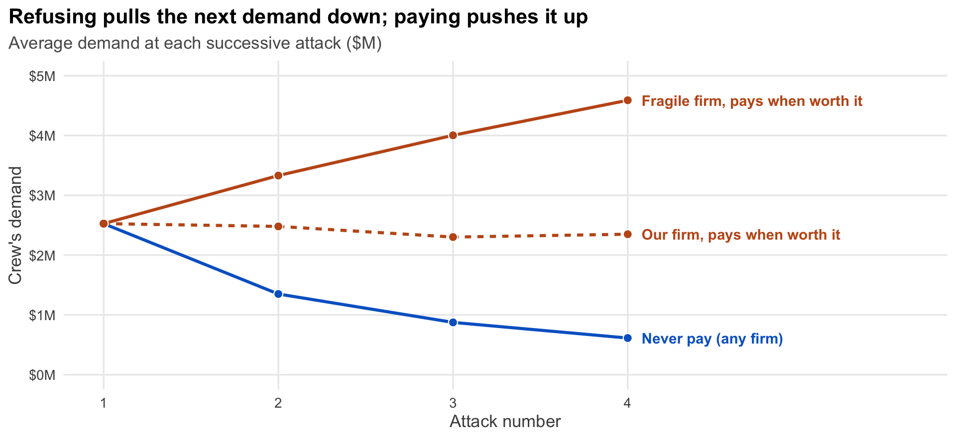
Each incident is also a lesson for the crew. A crew that is paid concludes we value our systems more than it guessed, and asks for more next time. A crew that is refused lowers its estimate, and its next demand falls. We simulate a 10-year horizon in which the crew learns from every incident and favors targets that have paid before. For a firm that never pays, lower demands are not the benefit; the benefit is that a crew expecting less attacks less often.
We compare two policies. **Pay when worth it** means paying whenever, in that incident, the demand is below our walk-away point. **Never pay** means refusing every time, committed in advance.
```{r}
#| label: fig-demand-path
#| fig-cap: "Average demand the crew posts at each successive attack, by firm and policy, at a 15% annual attack rate."
#| fig-alt: "Three lines over attacks one to four. Never pay falls steadily. Our firm, paying when worth it, stays roughly flat. The fragile firm, paying when worth it, rises with each attack."
#| fig-height: 4.6
base_grid <- at_p0(p0b)
dp <- bind_rows(
  tibble(series = "Never pay (any firm)", attack = 1:4, demand = rep$demand_seqs$R, policy = "never"),
  base_grid |> filter(policy == "rational", firm != "resilient") |>
    tidyr::pivot_longer(demand_1:demand_4, names_to = "attack", values_to = "demand") |>
    transmute(series = paste0(c(typical = "Our firm", fragile = "Fragile firm")[firm], ", pays when worth it"),
              attack = readr::parse_number(attack), demand, policy)
)
ends <- dp |> filter(attack == 4)
ggplot(dp, aes(attack, demand, color = policy, group = series)) +
  geom_line(aes(linetype = series), linewidth = 1.1) +
  geom_point(size = 2.8, color = "white") +
  geom_point(size = 2) +
  geom_text(data = ends, aes(label = series), hjust = 0, nudge_x = 0.08, size = 3.9, fontface = "bold") +
  scale_color_manual(values = POLICY_COLS, guide = "none") +
  scale_linetype_manual(values = c("solid", "solid", "22"), guide = "none") +
  scale_x_continuous("Attack number", breaks = 1:4, limits = c(1, 5.6)) +
  scale_y_continuous("Crew's demand", labels = \(x) paste0("$", x, "M"), limits = c(0, 5)) +
  labs(title = "Refusing pulls the next demand down; paying pushes it up",
       subtitle = "Average demand at each successive attack ($M)")
```
::: {.reader-note}
**How to read the plot.** Each line follows the crew's demand from the first attack to the fourth. The blue line is a firm that never pays; because the crew learns only from refusals, its path is the same for any firm. The orange lines are firms that pay when the demand is below their walk-away point: dashed for our firm, solid for the fragile one. Points are averages over the simulated paths that reach each attack.
**What the plot tells you.** Refusal teaches the crew that we are a poor prospect: its demand falls from `r fmt_m(rep$demand_seqs$R[1], 2)` to `r fmt_m(rep$demand_seqs$R[3], 2)` by the third attack. The fragile firm, which pays almost every time, sees demands climb to `r fmt_m(base_grid$demand_4[base_grid$firm == "fragile" & base_grid$policy == "rational"], 2)` by the fourth. In one survey, 78% of payers were attacked again and 63% of those were asked for more, though it does not compare payers with non-payers ([Infosecurity Magazine, February 2024](https://www.infosecurity-magazine.com/news/orgs-repeat-ransomware-paying/)).
:::
## Ten years of cost
How often we expect to be attacked is the input the board is least sure of, so the chart below lets you set it.
```{ojs}
//| echo: false
//| output: false
repRows = transpose(rep_grid)
firmLab = ({resilient: "Resilient", typical: "Our firm", fragile: "Fragile"})
polLab = ({never: "Never pay", rational: "Pay when worth it"})
xMax = Math.ceil(d3.max(repRows, d => d.cost_10y) / 5) * 5
```
```{ojs}
//| echo: false
viewof rate = Inputs.range([5, 25], {step: 1, value: 15, label: "Annual chance of a ransomware attack (%)"})
```
```{ojs}
//| echo: false
//| output: false
now = repRows.filter(d => Math.abs(d.p0 - rate / 100) < 1e-9)
  .filter(d => !(d.firm === "resilient" && d.policy === "rational"))
  .map(d => ({...d, firmL: firmLab[d.firm],
              polL: d.firm === "resilient" ? "Same under both policies" : polLab[d.policy]}))
pairs = ["typical", "fragile"].map(f => ({
  firmL: firmLab[f],
  x1: now.find(d => d.firm === f && d.policy === "never").cost_10y,
  x2: now.find(d => d.firm === f && d.policy === "rational").cost_10y
}))
```
```{ojs}
//| echo: false
//| label: fig-ten-year
//| fig-cap: "Expected 10-year cost by firm profile and policy at the selected annual attack rate. Labels give expected attacks over 10 years. The resilient firm never pays under either policy, so it is shown once."
Plot.plot({
  height: 340, marginLeft: 90, marginRight: 30, marginBottom: 45, marginTop: 20,
  style: {fontFamily: "inherit", fontSize: "13px"},
  x: {domain: [0, xMax], label: "Expected 10-year cost ($M)", labelAnchor: "center", grid: true},
  y: {domain: ["Resilient", "Our firm", "Fragile"], label: null},
  color: {domain: ["Never pay", "Pay when worth it", "Same under both policies"],
          range: ["#0166CC", "#C2571A", "#5A5A5A"], legend: true},
  marks: [
    Plot.link(pairs, {x1: "x1", x2: "x2", y1: "firmL", y2: "firmL", stroke: "#BBBBBB", strokeWidth: 3}),
    Plot.dot(now, {x: "cost_10y", y: "firmL", fill: "polL", r: 8, stroke: "white", strokeWidth: 2,
      channels: {Policy: "polL", "Attacks in 10 years": d => d.attacks_10y.toFixed(2)},
      tip: {format: {x: d => "$" + d.toFixed(1) + "M", fill: false, y: false}}}),
    Plot.text(now.filter(d => d.policy === "rational"), {x: "cost_10y", y: "firmL", dy: -18, fontSize: 12, fill: "#333",
      text: d => "$" + d.cost_10y.toFixed(1) + "M · " + d.attacks_10y.toFixed(1) + " attacks"}),
    Plot.text(now.filter(d => d.policy === "never"), {x: "cost_10y", y: "firmL", dy: 20, fontSize: 12, fill: "#333",
      text: d => "$" + d.cost_10y.toFixed(1) + "M · " + d.attacks_10y.toFixed(1) + " attacks"})
  ]
})
```
```{ojs}
//| echo: false
gap = f => now.find(d => d.firm === f && d.policy === "rational").cost_10y - now.find(d => d.firm === f && d.policy === "never").cost_10y
word = g => g >= 0 ? "saves" : "costs"
html`<div class="slider-sentence">At a <b>${rate}%</b> annual attack rate, a credible no-pay policy ${word(gap("typical"))} our firm about <b>$${Math.abs(gap("typical")).toFixed(1)}M</b> over 10 years and ${word(gap("fragile"))} the fragile firm about <b>$${Math.abs(gap("fragile")).toFixed(1)}M</b>.</div>`
```
```{=html}
<noscript>
```
```{r}
#| echo: false
#| fig-alt: "Static 10-year cost chart at a 15 percent annual attack rate."
#| fig-height: 3.6
tg <- base_grid |> filter(!(firm == "resilient" & policy == "rational")) |>
mutate(firmL = factor(FIRM_LABELS[firm], levels = rev(FIRM_LABELS)),
polL = if_else(firm == "resilient", "Same under both policies", POLICY_LABELS[policy]))
ggplot(tg, aes(cost_10y, firmL, color = polL)) +
geom_line(aes(group = firmL), color = "gray75", linewidth = 1.5) +
geom_point(size = 4) +
geom_text(aes(label = paste0(fmt_m(cost_10y), " · ", fmt_num(attacks_10y, 1), " attacks")),
nudge_y = 0.28, size = 3.5, color = "gray20") +
scale_color_manual(values = c(`Never pay` = "#0166CC", `Pay when worth it` = "#C2571A",
`Same under both policies` = "#5A5A5A"), name = NULL) +
labs(x = "Expected 10-year cost ($M)", y = NULL, title = "10-year cost at a 15% annual attack rate (static version)")
```
```{=html}
</noscript>
```
::: {.reader-note}
**How to read the plot.** Each row is a firm profile: resilient (4-day restore, 0.90 backup credibility), our firm (10 days, 0.80) and fragile (21 days, 0.60). Blue dots are never pay; orange dots pay when worth it. The resilient firm never pays under either policy, so it has one gray dot. Each label gives the expected 10-year cost and expected number of attacks. Drag the slider to change the annual chance of an attack.
**What the plot tells you.** At `r fmt_pct(p0b)`, never paying saves our firm about `r fmt_m(saving(p0b, "typical"))` and the fragile firm about `r fmt_m(saving(p0b, "fragile"))` over 10 years. The saving comes from fewer attacks: `r fmt_num(att_at(p0b, "fragile", "rational"), 1)` in 10 years for the fragile firm if it pays when worth it, against `r fmt_num(att_at(p0b, "fragile", "never"), 1)` if it never pays. The saving grows quickly with the attack rate. The resilient firm would refuse every demand anyway, so for it the policy costs nothing to keep.
:::
The more often you expect to be attacked, the more a reputation for refusing is worth. At a `r fmt_pct(min(P0_GRID))` annual rate, the fragile firm is slightly better off paying case by case (by `r fmt_m(-saving(min(P0_GRID), "fragile"))` over 10 years), because it is rarely attacked often enough for reputation to matter. From about `r fmt_pct(fragile_cross)` upward, never paying is cheaper for both firms.
## Why the policy must be credible
A no-pay policy is only worth what the crew believes about it, and a policy breaks under pressure when breaking it pays. In the moment, a fragile firm facing the first `r fmt_m(rep$opening, 2)` demand saves about `r fmt_m(fr$in_moment_saving)` by paying, because its walk-away point is `r fmt_m(fr$R_star, 2)`.
To test whether that temptation should win, we compare never paying with paying once, at the first incident, and never again. Costs are in present value at a `r fmt_pct(P$reputation$discount_rate)` discount rate, so the saving on the day counts in full and later attacks count for less. For the fragile firm, paying once costs `r fmt_m(pv_of(eta_b, "fragile", "deviate_once"))` over 10 years against `r fmt_m(pv_of(eta_b, "fragile", "never"))` for never paying: the extra attacks it invites outweigh the saving, so the policy is credible, by a margin of `r fmt_m(pv_of(eta_b, "fragile", "deviate_once") - pv_of(eta_b, "fragile", "never"))`. For our firm the margin is `r fmt_m(pv_of(eta_b, "typical", "deviate_once") - pv_of(eta_b, "typical", "never"))`. If crews ignore past payments, the result reverses: paying once saves the fragile firm `r fmt_m(pv_of(0, "fragile", "never") - pv_of(0, "fragile", "deviate_once"))`, and the policy is not credible.
A resilient firm faces no such test. Its walk-away point is `r fmt_m(prof$R_star[prof$profile == "resilient"], 2)`, so refusing is also its cheapest move on the day. Its policy is believed because it never has to be enforced against its own interest. Resilience is what turns a stated policy into a believed one.
## The assumption everything rests on
```{r}
#| label: tbl-eta
#| tbl-cap: "Expected 10-year cost ($M) by how strongly crews favor firms that have paid before, at a 15% annual attack rate."
rep$eta |>
  filter(eta %in% unlist(P$reputation$eta_table)) |>
  select(eta, firm, policy, cost_10y) |>
  tidyr::pivot_wider(names_from = c(firm, policy), values_from = cost_10y) |>
  gt() |>
  cols_label(eta = "Targeting response (η)",
             typical_rational = "Pay when worth it", typical_never = "Never pay",
             fragile_rational = "Pay when worth it", fragile_never = "Never pay") |>
  tab_spanner("Our firm", starts_with("typical")) |>
  tab_spanner("Fragile firm", starts_with("fragile")) |>
  fmt_number(columns = -eta, decimals = 1) |>
  fmt_number(columns = eta, decimals = 2) |>
  tab_style(cell_text(weight = "bold"),
            cells_body(columns = typical_never, rows = typical_never < typical_rational)) |>
  tab_style(cell_text(weight = "bold"),
            cells_body(columns = typical_rational, rows = typical_rational < typical_never)) |>
  tab_style(cell_text(weight = "bold"),
            cells_body(columns = fragile_never, rows = fragile_never < fragile_rational)) |>
  tab_style(cell_text(weight = "bold"),
            cells_body(columns = fragile_rational, rows = fragile_rational < fragile_never)) |>
  cols_align("center", -eta) |>
  gt_board()
```
::: {.reader-note}
**How to read the table.** Each row sets how strongly crews favor firms that have paid before. Zero means they don't care; one means a firm whose expected payout is twice as high is attacked twice as often. Each cell is the expected 10-year cost for one firm and policy, in $M. The cheaper policy in each row and firm is in bold.
**What the table tells you.** With no targeting response, paying when worth it is always cheaper, because it is the best choice in each incident by construction. Never paying wins once crews favor known payers: above about `r fmt_num(be_of("typical"), 2)` for our firm and `r fmt_num(be_of("fragile"), 2)` for the fragile firm. The whole reputation benefit rests on this one behavioral assumption. If crews ignore past payments, the case for never paying must rest on other grounds, such as sanctions risk.
:::
The case for a no-pay reputation rests on attackers favoring known payers. Industry surveys show that many payers are attacked again, but they do not report how often non-payers are, so the strength of this effect is unmeasured. It is the model's most important assumption.