---
title: "The Game"
subtitle: "How a ransomware incident plays out as a bargaining game"
---
```{r setup}
#| include: false
source("R/00_params.R"); source("R/01_utils.R"); source("R/90_theme.R")
library(dplyr); library(ggplot2); library(gt)
wa <- read_result("walkaway")
mc <- read_result("mc_drivers")
rep <- read_result("reputation")
sh <- mc$shares
share_of <- \(tgt, v) sh$share[sh$target == tgt & sh$input == v]
pay_parts <- cost_pay_parts(BASE, D_BASE)
ref_parts <- cost_refuse_parts(BASE)
sbd <- wa$staged_by_detect
tp_tot <- wa$two_paths |> summarise(total = sum(cost), .by = path)
```
*All money is in $M and all values are illustrative. The firm is synthetic.*
## The setup
A ransomware crew has encrypted the production platform of a 500-person fintech software firm and copied its client data. The crew posts a single demand. The firm can pay the demand, refuse and restore from backups, or combine the two: start restoring at once and pay only if the backups fail. The firm is a privately held company licensed by New York's Department of Financial Services (NYDFS), and several of its clients are listed companies.
Each side knows different things. The firm knows its own restore time and how much it trusts its backups. The crew doesn't; it can only guess from what it has seen of firms like ours. The crew wants the largest payment it can get, and the firm wants the cheaper path.
The data theft is treated separately from the encryption, because paying does not reliably buy silence. Coveware puts it bluntly: "threat actors' promises to delete stolen data cannot be verified" ([Coveware, October 2026](https://coveware.com/2026/10/the-silent-ransom-group-leak-shows-why-paying-for-silence-fails/)). Whichever path we choose, some chance of a public leak remains.
## Three paths
```{r}
#| label: fig-two-paths
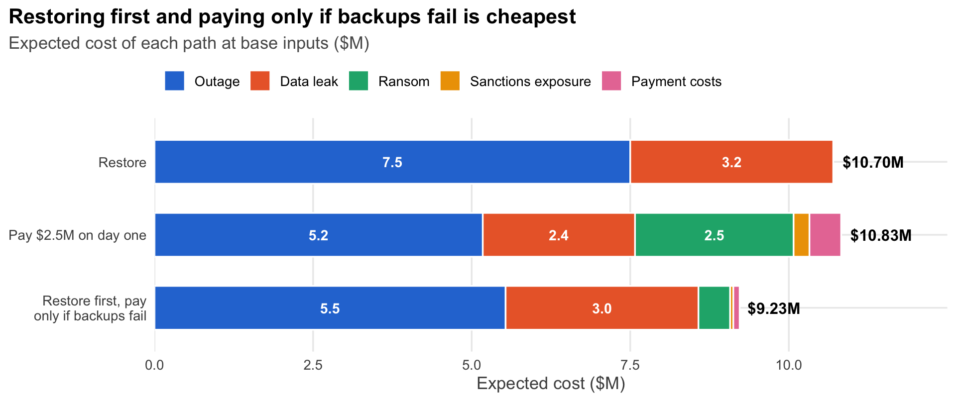
#| fig-cap: !expr paste0("Expected cost of three paths at base inputs and a ", fmt_m(D_BASE), " demand. The staged path assumes a failed restore is discovered after ", BASE$t_detect, " days.")
#| fig-alt: !expr paste0("Three horizontal stacked bars of expected cost. Restoring costs ", fmt_m(wa$C_refuse, 2), ", paying on day one costs ", fmt_m(wa$C_pay, 2), ", and restoring first while paying only if backups fail costs ", fmt_m(wa$C_staged, 2), ". Outage is the largest component of every path.")
#| fig-height: 4.2
comp_order <- c("Outage", "Data leak", "Ransom", "Sanctions exposure", "Payment costs")
tp <- wa$two_paths |>
  mutate(
    component = factor(COMPONENT_LABELS[component], levels = rev(comp_order)),
    path = factor(path, levels = rev(unique(path)))
  )
totals <- tp |> summarise(total = sum(cost), .by = path)
ggplot(tp, aes(cost, path, fill = component)) +
  geom_col(width = 0.6, color = "white", linewidth = 0.6) +
  geom_text(aes(label = if_else(cost >= 0.9, fmt_num(cost, 1), "")),
            position = position_stack(vjust = 0.5), size = 3.8, color = "white", fontface = "bold") +
  geom_text(data = totals, aes(total, path, label = fmt_m(total, 2)), inherit.aes = FALSE,
            hjust = -0.15, size = 4.2, fontface = "bold") +
  scale_fill_manual(values = COMPONENT_COLS, breaks = comp_order, name = NULL) +
  scale_x_continuous("Expected cost ($M)", limits = c(0, 12.5), breaks = seq(0, 10, 2.5), expand = c(0, 0)) +
  scale_y_discrete(labels = scales::label_wrap(22)) +
  labs(y = NULL,
       title = "Restoring first and paying only if backups fail is cheapest",
       subtitle = "Expected cost of each path at base inputs ($M)")
```
::: {.reader-note}
**How to read the plot.** Each bar is one path, built from the costs we expect along it. The colored segments show where the money goes: lost operations while systems are down, a possible public leak of client data and, where a payment is made, the ransom, the sanctions penalty risk and the legal and filing costs of paying. The bottom bar starts restoring at once and pays only if the backups turn out to have failed, so its payment costs are small.
**What the plot tells you.** Restoring costs `r fmt_m(wa$C_refuse, 2)` and paying on day one `r fmt_m(wa$C_pay, 2)`, about `r fmt_pct(abs(wa$C_pay / wa$C_refuse - 1))` apart, well inside the model's uncertainty. Restoring first and paying only if backups fail costs `r fmt_m(wa$C_staged, 2)`, less than either. Paying on day one shortens the outage but does not end it: the decryptor sometimes fails, and decryption itself takes days. The staged path wins because the ransom is paid only in the minority of incidents where backups fail.
:::
The staged path wins because it turns a payment into a fallback for backup failure. With backup credibility of `r fmt_num(BASE$b, 2)`, a payment comes into question in only `r fmt_pct(1 - BASE$b)` of incidents, so backup credibility decides whether a payment is ever needed. The path stays cheapest even if a failed restore takes `r max(sbd$t_detect)` days to discover (`r fmt_m(sbd$cost[sbd$t_detect == max(sbd$t_detect)], 2)`), and is the cheapest of the three in `r fmt_pct(mc$summary$staged_cheapest_share)` of simulated incidents. It assumes the firm can negotiate while restoring; leak deadlines or rising demands can remove that option.
The firm's **walk-away point** is the largest demand worth paying on day one, before any restore has been tried; the decision maps on this site describe that day-one choice. At the most likely values it is `r fmt_m(wa$R_base, 2)`, just below the `r fmt_m(D_BASE)` demand, so the firm is close to indifferent. Allowing for uncertainty in every input, paying a `r fmt_m(D_BASE)` demand on day one is cheaper than restoring in `r fmt_pct(mc$summary$p_pay_at_base_demand)` of simulated incidents: with today's restore times, this firm is often a rational payer. Each day cut from restore time lowers the walk-away point by about `r fmt_m(wa$slope, 2)`. About `r fmt_m(wa$leak_part, 2)` of it assumes that paying lowers the chance of a leak; if it does not, the walk-away point falls to `r fmt_m(wa$R_star_no_leak_benefit, 2)`.
## The inputs
```{r}
#| label: tbl-inputs
#| tbl-cap: "Model inputs: base values and the ranges used in the Monte Carlo."
meta <- readr::read_csv(file.path(PROJECT_ROOT, "data", "inputs.csv"), show_col_types = FALSE)
range_txt <- function(spec) {
  par <- unlist(spec$par)
  switch(spec$dist,
    tri = sprintf("Triangular: %g to %g, most likely %g", par[1], par[3], par[2]),
    beta = sprintf("Beta(%g, %g), mean %.2f", par[1], par[2], par[1] / sum(par)),
    fixed = "Fixed",
    ratio_of_p_np = sprintf("p<sub>np</sub> × triangular(%g, %g, %g)", par[1], par[2], par[3])
  )
}
meta |>
  mutate(
    base = purrr::map_dbl(symbol, \(s) BASE[[s]]),
    range = purrr::map_chr(symbol, \(s) range_txt(INPUT_SPEC[[s]])),
    source = if_else(is.na(url), grounding, paste0("[", grounding, "](", url, ")"))
  ) |>
  select(label, meaning, unit, base, range, source) |>
  gt() |>
  fmt_markdown(columns = c(label, range, source)) |>
  fmt_number(columns = base, decimals = 2, drop_trailing_zeros = TRUE) |>
  cols_label(label = "Symbol", meaning = "Meaning", unit = "Unit", base = "Base",
             range = "Monte Carlo range", source = "Grounding") |>
  cols_align("right", base) |>
  gt_board()
```
::: {.reader-note}
**How to read the table.** Each row is one input to the cost model. The base column is the single value used for the worked example above. The range column is how uncertain we are: a triangular range gives the lowest, highest and most likely values, and a Beta range describes a probability with its average. The last column says where the value comes from; "Firm assumption" means it is set for this synthetic firm.
**What the table tells you.** Most inputs are judgments that the firm would replace with its own figures, especially outage cost per day and restore time. Probabilities such as backup credibility and decryptor reliability are uncertain, which is why the site tests the whole range rather than one point. The Governance page lists who would own each assumption and what should trigger a review.
:::
::: {.callout-note collapse="true" icon="false"}
## The walk-away formula
Expected outage if we refuse, where backups work with probability $b$:
$$E[T] = b\,T_r + (1-b)\,T_{fail}$$
Expected cost of refusing:
$$C_{refuse} = c\,E[T] + p_{np}K_{leak}$$
Expected cost of paying demand $D$. The decryptor works with probability $q$; otherwise we fall back to restoring:
$$C_{pay}(D) = D(1+s\kappa) + K_{pay} + c\,[\,d_{pay} + q\,T_d + (1-q)\,E[T]\,] + p_p K_{leak}$$
Pay only if $C_{pay}(D) \le C_{refuse}$. Solving for $D$ gives the walk-away point:
$$R^* = \frac{c\,[\,q\,(E[T]-T_d) - d_{pay}\,] + (p_{np}-p_p)\,K_{leak} - K_{pay}}{1+s\kappa}$$
The demand $D$ does not appear in $R^*$; it only decides which side of the line we fall on. $R^*$ rises in a straight line with restore time, with slope $c\,q\,b/(1+s\kappa)$. If $R^* \le 0$, paying is never worth it.
:::
## What the crew knows
The crew doesn't know our walk-away point, so it sets its demand from what it believes about firms like ours, mainly how long they take to restore. It picks the demand that maximizes its expected take: a higher demand earns more when paid but is refused more often. With the belief used here, its opening demand is `r fmt_m(rep$opening, 2)`. We set the crew's starting belief as a firm assumption at the high end of published figures: the median demand across all victims was $1.32M ([Sophos, State of Ransomware 2025](https://assets.sophos.com/X24WTUEQ/at/9brgj5n44hqvgsp5f5bqcps/sophos-state-of-ransomware-2025.pdf)), and Coveware's median payment in Q3 2026 was $400K ([Coveware, October 2026](https://coveware.com/2026/10/the-silent-ransom-group-leak-shows-why-paying-for-silence-fails/)).
The demand reflects what the crew believes about our restore time, not what our data is worth. Visible resilience lowers the opening number.
## What moves the decision
```{r}
#| label: fig-drivers
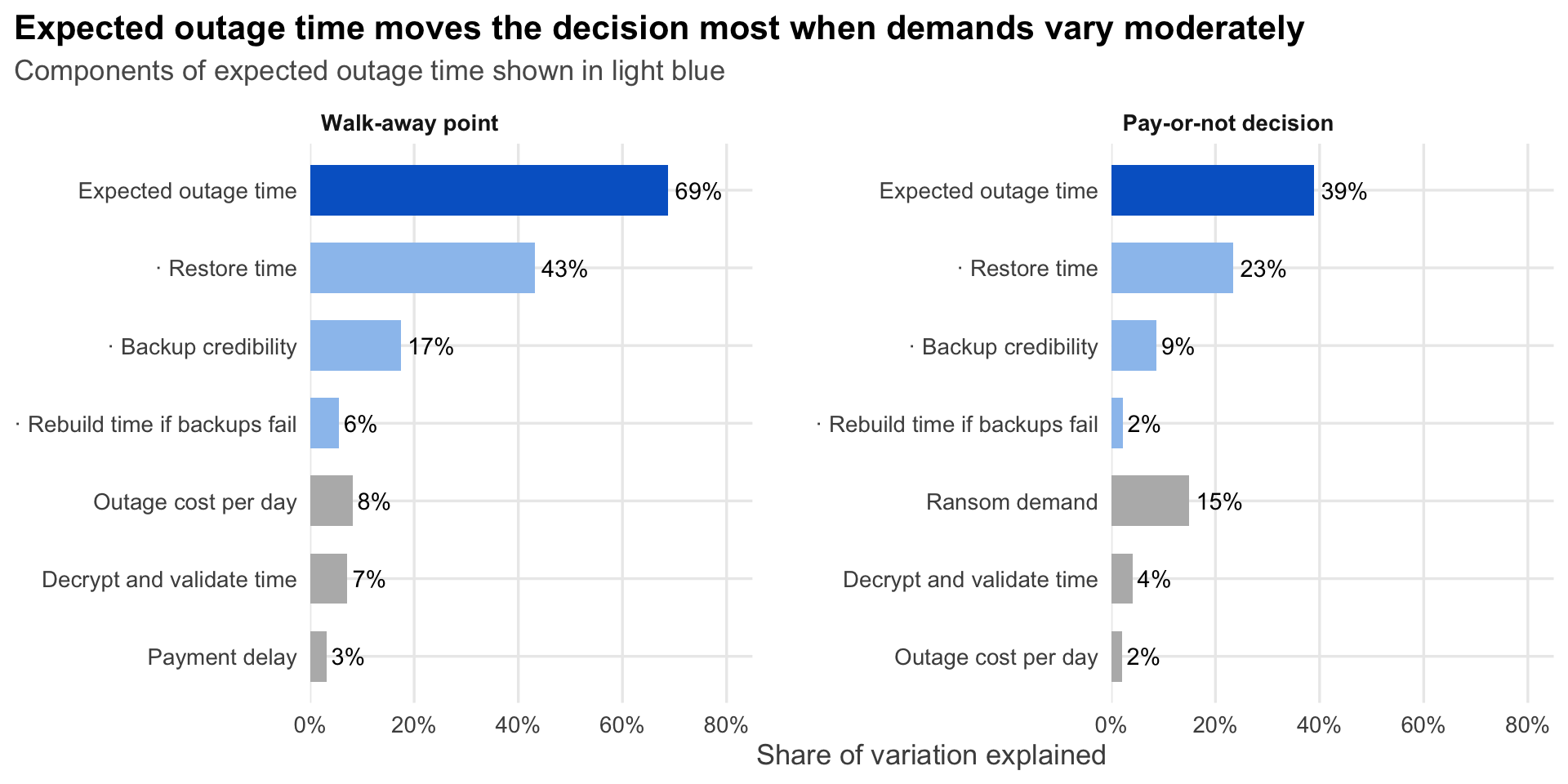
#| fig-cap: "Share of the variation in the walk-away point, and in the pay-or-not decision, explained by each input on its own; 200,000 simulated incidents. First-order shares show ranking only; interactions are not shown."
#| fig-alt: !expr paste0("Two panels of horizontal bars. Expected outage time explains ", fmt_pct(share_of("R_star", "E_T")), " of the walk-away point and ", fmt_pct(share_of("pay", "E_T")), " of the pay decision. Its components, restore time, backup credibility and rebuild time, are shown beneath it in light blue. The ransom demand explains ", fmt_pct(share_of("pay", "D")), " of the pay decision.")
#| fig-height: 5
facet_lab <- c(R_star = "Walk-away point", pay = "Pay-or-not decision")
comps <- c("T_r", "b", "T_fail")
d <- purrr::map(names(facet_lab), \(tg) {
  x <- sh |> filter(target == tg)
  others <- x |> filter(!input %in% c("E_T", comps)) |> slice_max(share, n = 3)
  bind_rows(filter(x, input == "E_T"), filter(x, input %in% comps) |> arrange(desc(share)), others) |>
    mutate(role = c("total", rep("component", 3), rep("other", 3)),
           lab = if_else(role == "component", paste0("\u00b7 ", DRIVER_LABELS[input]), DRIVER_LABELS[input]),
           key = paste(lab, tg, sep = "___"))
}) |> purrr::list_rbind() |>
  mutate(facet = factor(facet_lab[target], levels = facet_lab),
         key = factor(key, levels = rev(key)))
ggplot(d, aes(share, key, fill = role)) +
  geom_col(width = 0.65) +
  geom_text(aes(label = fmt_pct(share)), hjust = -0.15, size = 3.8) +
  facet_wrap(~facet, scales = "free_y") +
  scale_y_discrete(labels = \(x) sub("___.*", "", x)) +
  scale_fill_manual(values = c(total = "#0166CC", component = "#9CC3EE", other = "#B8B8B8"), guide = "none") +
  scale_x_continuous("Share of variation explained", labels = scales::label_percent(),
                     limits = c(0, 0.85), expand = c(0, 0)) +
  labs(y = NULL,
       title = "Expected outage time moves the decision most when demands vary moderately",
       subtitle = "Components of expected outage time shown in light blue") +
  theme(panel.spacing.x = unit(2, "lines"), strip.text = element_text(face = "bold", hjust = 0))
```
::: {.reader-note}
**How to read the plot.** We simulated `r fmt_num(N_MC, 0)` incidents, drawing every input from its range and the demand from a moderate spread. Each bar shows how much of the spread in the result one input explains on its own. The left panel is the walk-away point; the right is the yes-or-no pay decision. Expected outage time (dark blue) combines the three light-blue inputs beneath it, so those bars overlap it; read the chart as a ranking, not as parts of a whole.
**What the plot tells you.** Expected outage time explains `r fmt_pct(share_of("R_star", "E_T"))` of the variation in the walk-away point, and restore time alone `r fmt_pct(share_of("R_star", "T_r"))`. In the pay decision, expected outage time explains `r fmt_pct(share_of("pay", "E_T"))` and the demand `r fmt_pct(share_of("pay", "D"))`. That ranking depends on how widely demands vary: if they vary as much as published payments do, the demand comes first (see the [Governance](governance.qmd#sensitivity) page). Either way, restore time sets the threshold the demand is tested against.
:::
## The regulatory clock
Paying adds legal exposure; it never removes disclosure. OFAC can impose civil penalties "based on strict liability", so a sanctions link that surfaces after payment is still a violation ([OFAC, 2021](https://ofac.treasury.gov/media/912981/download)). As an NYDFS-covered entity, the firm must report an extortion payment within 24 hours. Within 30 days it must explain in writing why it was necessary, which alternatives were considered and what sanctions diligence was done ([23 NYCRR 500.17(c), ComplianceForge summary](https://complianceforge.com/ny-dfs-23-nycrr-500/23-nycrr-500-17-notices-to-superintendent); [DFS filing instructions](https://www.dfs.ny.gov/system/files/documents/2026/07/Reporting-an-Extortion-Payment_1.pdf)). The firm is not listed, but its listed clients run their own clock: if a client judges the incident material to it, that client's Form 8-K, Item 1.05, is due "within four business days" of the determination, whether or not anyone pays ([SEC](https://www.sec.gov/corpfin/cybersecurity)).