Question 2: Does It Beat a Simple Model?

The question

Does VendorScore forecast NorthPoint’s monthly incident total better than a plain 12-month rolling average of past counts, and does any advantage survive the deterioration in vendor patching after month 36? This tests one use of the model, aggregate monthly count forecasting. VendorScore may have other value, such as ranking vendors for attention, which this comparison does not price.

Method in brief

Each forecast is made at the start of month t for the incidents that will occur during that month. VendorScore’s forecast is the sum of its 300 vendor scores. The benchmark is the mean of actual counts in months t − 12 to t − 1. We assume each month’s patch latency and financial health are observed at the start of that month; if they were end-of-month measures, this would be a contemporaneous assessment, not a one-step-ahead forecast. We use raw scores over months 31 to 48, so no fitting touches the target months.

We summarise accuracy with mean squared error (MSE, in squared incidents) and mean absolute error (MAE, in incidents). We test equal accuracy with the Diebold–Mariano test from forecastdom:¹ a positive statistic means lower squared loss for VendorScore. We run it over months 31 to 48 and over months 37 to 48. With 18 and 12 observations the test has low power, and a small-sample correction does not cure a deliberately shifting environment, where loss patterns may not be stable.

Findings

ggplot(long, aes(month, value, colour = series, linetype = series)) +
  geom_vline(xintercept = fc$shift_month, colour = "grey50", linetype = "dotted") +
  geom_line(linewidth = 0.9) +
  geom_point(data = subset(long, series == "Actual incidents"), size = 2) +
  scale_colour_manual(values = c("Actual incidents" = okabe_ito[["blue"]],
                                 "VendorScore forecast" = okabe_ito[["orange"]],
                                 "12-month average" = okabe_ito[["grey"]])) +
  scale_linetype_manual(values = c("Actual incidents" = "solid",
                                   "VendorScore forecast" = "solid",
                                   "12-month average" = "longdash")) +
  labs(x = "Month", y = "Incidents per month (portfolio)", colour = NULL, linetype = NULL)

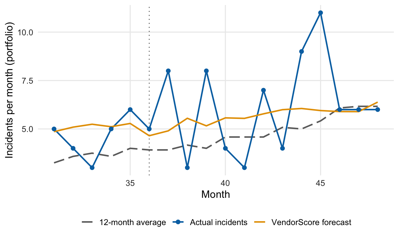
Figure 1: Monthly incident totals versus both forecasts, months 31–48. The vertical line marks month 36, the last month before patching latency drifts.

How to read the plot. Blue dots joined by a line are the actual incident counts across all 300 vendors. The orange line is VendorScore’s forecast and the grey dashed line is the 12-month average. The dotted line marks when patching began to slow.

What the plot tells you. Actual counts trend upward and swing widely. The 12-month average trails the trend and forecasts too low for most of the window, by 1.2 incidents a month on average. VendorScore’s average miss is 0.2. Both are conditional expected counts, not predictions of every fluctuation.

ggplot(tst, aes(month, cum_diff)) +
  geom_hline(yintercept = 0, colour = "grey50") +
  geom_vline(xintercept = fc$shift_month, colour = "grey50", linetype = "dotted") +
  geom_area(fill = okabe_ito[["blue"]], alpha = 0.18) +
  geom_line(colour = okabe_ito[["blue"]], linewidth = 1) +
  labs(x = "Month", y = "Cumulative advantage (squared incidents)")

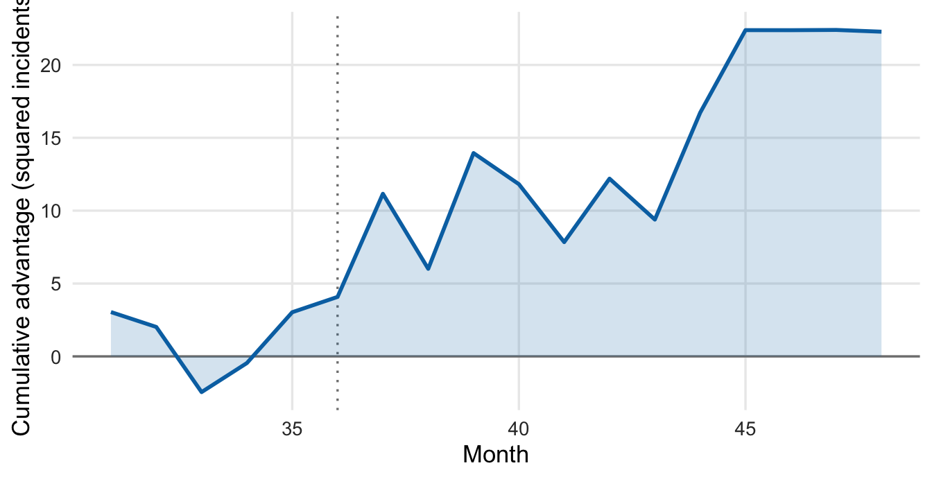
Figure 2: Cumulative loss differential, months 31–48: running sum of benchmark minus VendorScore squared error (squared incidents). Above zero favours VendorScore.

How to read the plot. Each month we ask which forecast was closer. The line is the running total, rising when VendorScore wins and falling when the 12-month average wins.

What the plot tells you. The line ends 22.3 above zero, with 4.1 accumulated by month 36 and 18.2 after it. It climbs unevenly, with several losing months, so this is a mixed record with a favourable tilt, not a steady edge.

tab <- data.frame(
  Window = c("Months 31–48 (n = 18)", "Months 37–48 (n = 12)"),
  `MSE, 12-month (incidents²)` = res$mse_naive, `MSE, VendorScore (incidents²)` = res$mse_vs,
  `MAE, 12-month (incidents)` = res$mae_naive, `MAE, VendorScore (incidents)` = res$mae_vs,
  `DM statistic` = res$dm_stat, `p-value` = res$dm_p, check.names = FALSE)
knitr::kable(tab, digits = c(0, 2, 2, 2, 2, 2, 3))

Table 1: Forecast accuracy and Diebold–Mariano tests. Positive statistic: lower squared loss for VendorScore.

Window	MSE, 12-month (incidents²)	MSE, VendorScore (incidents²)	MAE, 12-month (incidents)	MAE, VendorScore (incidents)	DM statistic	p-value
Months 31–48 (n = 18)	5.67	4.44	1.80	1.61	1.23	0.235
Months 37–48 (n = 12)	7.59	6.08	2.08	2.03	1.07	0.309

How to read the table. Each row is a stretch of months. The MAE columns show the average miss in incidents per month; the MSE columns square each miss, so large misses count more. The last two columns test whether the accuracy gap is bigger than expected if both forecasts were equally good.

What the table tells you. VendorScore has lower errors in both windows. The p-value is the chance of a loss difference at least this extreme if expected accuracy were equal and the test’s assumptions held; 0.235 and 0.309 are not small. That means no detectable advantage here, not proof of equality.

VendorScore’s MSE is 22% lower over the full window and 20% lower after the shift, while its MAE advantage nearly vanishes after the shift (2.03 versus 2.08). The vendor’s claimed AUC of 0.81 comes from its own development data. It cannot show whether VendorScore stays reliable at this bank once conditions change. Only the bank’s own ongoing monitoring can (§VII).

So What?

On this evidence VendorScore gets the level of incidents closer than the simple benchmark does, but the advantage is statistically unproven and concentrated in a period when the benchmark lagged a rising trend. The comparison covers aggregate counts, not vendor rankings.

The April 17, 2026 interagency Supervisory Guidance on Model Risk Management (Federal Reserve, FDIC, OCC) lists out-of-sample and out-of-time testing under model testing (§IV), and benchmarking and ongoing monitoring under validation (§V). The cumulative-differential chart fits there: a line a committee can watch. This is partial validation: it tests outputs, not the method.

Actionable Insights

Sound practice suggests benchmarking every vendor model against a named simple alternative, out of sample and out of time, and adding the loss differential to ongoing monitoring so that deterioration triggers review.

Footnotes

1. forecastdom 0.1.0, dm_test() with h = 1, squared-error loss, two-sided alternative, Harvey–Leybourne–Newbold correction (reference distribution t with n − 1 degrees of freedom), benchmark errors first. At h = 1 the package’s variance is the sample variance of the loss differences divided by n, with no autocorrelation adjustment.